# (launch:thebe)=
# # Defining a finite element ({term}`FE`)
#
# The finite element method is a way of representing a function $u$ in a function space $V$, given $u$
# satisfies a certain partial differential equation.
#
# In this tutorial, we will keep to function spaces $V\subset H^{1}(\Omega)$,
#
# $$
# H^1(\Omega):=\{u\in L^2(\Omega) \text{ and } \nabla u\in L^2(\Omega)\}.
# $$
#
# Next, we need a finite subset of functions in $H^1(\Omega)$, and we call this the finite element space.
# This means that any function in $V$ can be represented as a linear combination of these basis functions
#
# $$u\in V \Leftrightarrow u(x) = \sum_{i=0}^{N-1} u_i \phi_i(x),$$
# where $N$ are the number of basis functions, $\phi_i$ is the $i$-th basis function and $u_i$ are the coefficients.
#
#
# ## Formal definition of a finite element
# A finite element is often described{cite}`ciarlet2002` as a triplet $(R, \mathcal{V}, \mathcal{L})$ where
# - $R\subset \mathbb{R}^n$ is the reference element (often polygon or polyhedron).
# - $\mathcal{\mathcal{V}}$ is a finite-dimensional polynomial space on $R$ with dimension $n$.
# - $\mathcal{L}=\{l_0, \dots, l_{n-1}\}$ is the basis of the dual space
#   $\mathcal{V}^*:=\{f:\mathcal{V}\rightarrow\mathbb{R}\vert f \text{ is linear}\}.$
#
# One often associates each $l_i$ with a sub-entity of $R$, i.e. a vertex, an edge, a face or the cell itself.
#
# ## Example: A second order Lagrange space on a quadrilateral
#
# ```{sidebar}
# <center>
# <img src="https://defelement.com/img/element-Q-variant-equispaced-quadrilateral-2-dofs.png"
# width="250" height="250" /><br>
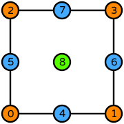
# Illustration of dof positioning on a quadrilateral
# (from <a href=https://defelement.com/img/element-Q-variant-equispaced-quadrilateral-2-dofs.html>DefElement</a>, CC BY 4.0).
# </center>
# ```
#
# - $R$ is a quadrilateral with vertices $(0,0)$, $(1,0)$, $(0,1)$ and $(1,1)$.
# - $\mathcal{V}=\mathrm{span}\{1, y, y^2, x, x^2, xy, xy^2, x^2, x^2y, x^2y^2\}$.
# - The basis of the dual space is
#
# $$
# \begin{align*}
#   l_0&: v \mapsto v(0,0)\\
#   l_1&: v \mapsto v(1,0)\\
#   l_2&: v \mapsto v(0,1)\\
#   l_3&: v \mapsto v(1,1)\\
#   l_4&: v \mapsto v(0.5,0)\\
#   l_5&: v \mapsto v(0, 0.5)\\
#   l_6&: v \mapsto v(1, 0.5)\\
#   l_7&: v \mapsto v(0.5, 1)\\
#   l_8&: v \mapsto v(0.5, 0.5)\\
# \end{align*}
# $$
#

# ## Determining the underlying basis functions $\phi_i$
#
# The basis functions are determined by
#
# $$l_i(\phi_j)=\delta_{ij}=\begin{cases}1 \qquad i=j\\ 0 \qquad i \neq j\end{cases}$$
#
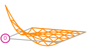
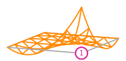
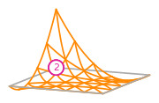
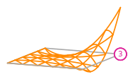
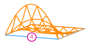
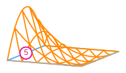
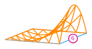
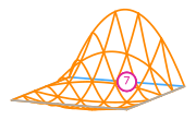
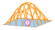
# For the example above this gives us the following basis functions
#
#
# <center>
# <img src="https://defelement.com/img/element-Q-variant-equispaced-quadrilateral-2-0.png"
# width="202" height="115" />
# <img src="https://defelement.com/img/element-Q-variant-equispaced-quadrilateral-2-1.png"
# width="202" height="115" />
# <img src="https://defelement.com/img/element-Q-variant-equispaced-quadrilateral-2-2.png"
# width="202" height="115" />
# <img src="https://defelement.com/img/element-Q-variant-equispaced-quadrilateral-2-3.png"
# width="202" height="115" />
# <img src="https://defelement.com/img/element-Q-variant-equispaced-quadrilateral-2-4.png"
# width="202" height="115" />
# <img src="https://defelement.com/img/element-Q-variant-equispaced-quadrilateral-2-5.png"
# width="202" height="115" />
# <img src="https://defelement.com/img/element-Q-variant-equispaced-quadrilateral-2-6.png"
# width="202" height="115" />
# <img src="https://defelement.com/img/element-Q-variant-equispaced-quadrilateral-2-7.png"
# width="202" height="115" />
# <img src="https://defelement.com/img/element-Q-variant-equispaced-quadrilateral-2-8.png"
# width="202" height="115" />
# <br>
# The basis functions of a second order Lagrange space on a quadrilateral
# (from <a href=https://defelement.com/elements/examples/quadrilateral-lagrange-equispaced-2.html>DefElement</a>, CC BY 4.0).
# <br>
# </center>
#
# ### Uniqueness of basis functions
# This means that we can use different basis functions to span the same polynomial spaces $\mathcal{V}$
# by choosing different dual basis functions $l_i$.
#
# An example of this is choosing different positioning of the dofs (non-equispaced) for Lagrange elements.
# See [FEniCS: Variants of Lagrange Elements](https://docs.fenicsproject.org/dolfinx/v0.9.0/python/demos/demo_lagrange_variants.html)
# for more information.
#
# An algorithmic approach for determining the basis functions based of the dual space is for instance given at
# [Finite elements - analysis and implementation
# (Imperial College London)](https://finite-element.github.io/L2_fespaces.html#vandermonde-matrix-and-unisolvence).
#
# # Creating a finite element in FEniCSx
#
# There is a large variety of finite elements: [List of finite elements](https://defelement.com/elements/index.html).
#
# However, in today's lecture, we will focus on the [Lagrange elements](https://defelement.com/elements/lagrange.html).
#
# We start by considering the basis functions of a first order Lagrange element on a triangle:
#
# <center>
# <img src="https://defelement.com/img/element-Lagrange-variant-equispaced-triangle-1-0-large.png"
# width="150" height="150" />
# <img src="https://defelement.com/img/element-Lagrange-variant-equispaced-triangle-1-1-large.png"
# width="150" height="150" />
# <img src="https://defelement.com/img/element-Lagrange-variant-equispaced-triangle-1-2-large.png"
# width="150" height="150" /><br>
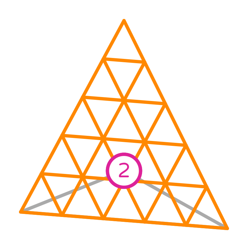
# First order Lagrange basis functions<br><br>
# </center>

#
# To symbolically represent this element, we use `basix.ufl.element`,
# that creates a representation of a finite element using {term}`Basix`,
# which in turn can be used in the {term}`UFL`.

# +
import numpy as np

import basix.ufl

element = basix.ufl.element("Lagrange", "triangle", 1)

# -
# The three arguments we provide to Basix are the name of the element family, the reference
# cell we would like to use and the degree of the polynomial space.
#

# Next, we will evaluate the basis functions at a certain set of `points` in the reference triangle.
# We call this {term}`tabulation` and we use the `tabulate` method of the element object.
# The two input arguments are:
# 1) The number of spatial derivatives of the basis functions we want to compute.
# 2) A set of input points to evaluate the basis functions at as
# a numpy array of shape `(num_points, reference_cell_dimension)`.
#
# In this case, we want to compute the basis functions themselves, so we set the first argument to 0.

# +
points = np.array([[0.0, 0.1], [0.3, 0.2]])
values = element.tabulate(0, points)
# -

# + tags = ["remove-input"]
print(f"{values=}")
# -

# We can get the first order derivatives of the basis functions by setting the first argument to 1.
# Observe that the output we get from this command also includes the 0th order derivatives.
# Thus we note that the output has the shape `(num_spatial_derivatives+1, num_points, num_basis_functions)`

# +
values = element.tabulate(1, points)
# -

# + tags = ["remove-input"]
print(values)
# -

# ## Visualizing the basis functions

# Next, we create a short script for visualizing the basis functions on the reference element.
# We will for simplicity only consider first order derivatives and triangular or quadrilateral cells.

import matplotlib.pyplot as plt


def plot_basis_functions(element, M: int):
    """Plot the basis functions and the first order derivatives sampled at
    `M` points along each direction of an edge of the reference element.

    :param element: The basis element
    :param M: Number of points
    :return: The matplotlib instances for a plot of the basis functions
    """
    # We use basix to sample points (uniformly) in the reference cell
    points = basix.create_lattice(element.cell_type, M - 1, basix.LatticeType.equispaced, exterior=True)

    # We evaluate the basis function and derivatives at the points
    values = element.tabulate(1, points)

    # Determine the layout of the plots
    num_basis_functions = values.shape[2]
    num_columns = values.shape[0]

    derivative_dir = ["x", "y"]
    figs = [
        plt.subplots(1, num_columns, layout="tight", subplot_kw={"projection": "3d"})
        for i in range(num_basis_functions)
    ]
    colors = plt.rcParams["axes.prop_cycle"]()
    for i in range(num_basis_functions):
        _, axs = figs[i]
        [(ax.set_xlabel("x"), ax.set_ylabel("y")) for ax in axs.flat]
        for j in range(num_columns):
            ax = axs[j]
            ax.scatter(points[:, 0], points[:, 1], values[j, :, i], color=next(colors)["color"])
            if j > 0:
                ax.set_title(
                    r"$\partial\phi_{i}/\partial {x_j}$".format(i="{" + f"{i}" + "}", x_j=derivative_dir[j - 1])
                )
            else:
                ax.set_title(r"$\phi_{i}$".format(i="{" + f"{i}" + "}"))
    return figs


# ## Basis functions sampled at random points

fig = plot_basis_functions(element, 15)

# We also illustrate the procedure on a second order Lagrange element on a quadrilateral, as discussed above.

second_order_element = basix.ufl.element("Lagrange", "quadrilateral", 2, basix.LagrangeVariant.gll_warped)
fig = plot_basis_functions(second_order_element, 12)

# ## Lower precision tabulation
#
# In some cases, one might want to use a lower accuracy for tabulation of basis functions to speed up computations.
# This can be changed in basix by adding `dtype=np.float32` to the element constructor.

low_precision_element = basix.ufl.element("Lagrange", "triangle", 1, dtype=np.float32)
points_low_precision = points.astype(np.float32)
basis_values = low_precision_element.tabulate(0, points_low_precision)
print(f"{basis_values=}\n   {basis_values.dtype=}")

# We observe that elements that are close to zero is now an order of magnitude larger than its `np.float64` counterpart.

# ## Exercises
#
# Basix allows for a large variety of extra options to tweak your finite elements, see for instance
# [Variants of Lagrange elements](https://docs.fenicsproject.org/dolfinx/v0.9.0/python/demos/demo_lagrange_variants.html)
# for how to choose the node spacing in a Lagrange element.
# Using the plotting script above, try to plot basis functions of a high order quadrilateral element with different Lagrange variants.
# - Do you observe the same phenomenon on quadrilaterals as on intervals?
# - What about triangles?
#
# ```{admonition} Tip
# :class: dropdown tip
# Try to increase the plotting resolution to 40.
# ```

# ## References
# ```{bibliography}
#    :filter: cited and ({"src/finite_element_method/finite_element"} >= docnames)
# ```