Mesh creation in serial and parallel#
Author: Jørgen S. Dokken
In this tutorial we will consider the first important class in DOLFINx, the dolfinx.mesh.Mesh class.
A mesh consists of a set of cells. These cells can be intervals, triangles, quadrilaterals, hexahedrons or tetrahedrons. Each cell is described by a set of coordinates, and its connectivity.
Mesh creation from numpy arrays#
For instance, let us consider a unit square. If we want to discretize it with triangular elements, we could create the set of vertices as a \((4\times 2)\) numpy array
import numpy as np

tri_points = np.array([[0, 0], [0, 1], [1, 0], [1, 1]], dtype=np.float64)
Next, we have to decide on how we want to create the two triangles in the mesh. Let’s choose the first cell to consist of vertices \(0,1,3\) and the second cell consist of vertices \(0,2,3\)
triangles = np.array([[0, 1, 3], [0, 2, 3]], dtype=np.int64)
We note that for triangular cells, we could order the vertices in any order say [[1,3,0],[2,0,3]], and the mesh would equivalent.
Some finite element software reorder cells to ensure consistent integrals over interior facets.
In DOLFINx, another strategy has been chosen, see [SDRW22] for more details.
Let’s consider the unit square again, but this time we want to discretize it with two quadrilateral cells.
quad_points = np.array(
    [[0, 0], [0.3, 0], [1, 0], [0, 1], [0.5, 1], [1, 1]], dtype=np.float64
)
quadrilaterals = np.array([[0, 1, 3, 4], [1, 2, 4, 5]], dtype=np.int64)
Note that we do not parse the quadrilateral cell in a clockwise or counter-clockwise fashion. Instead, we are using a tensor product ordering. The ordering of the sub entities all cell types used in DOLFINx can be found at Basix supported elements. We also note that this unit square mesh has non-affine elements.
Next, we would like to generate the mesh used in DOLFINx. To do so, we need to generate the coordinate element. This is the paramterization of each an every element, and the only way of going between the physical element and the reference element. We will denote any coordinate on the reference element as \(\mathbf{X}\), and any coordinate in the physical element as \(\mathbf{x}\), with the mapping \(M\) such that \(\mathbf{x} = M(\mathbf{X})\).
We can write
where \(\mathbf{v}_i\) is the \(i\)th vertex of a cell and \(\phi_i\) are the basis functions specifed at DefElement P1 triangles and DefElement Q1 quadrilaterals.
In DOLFINx we use the Unified Form Language to define finite elements.
Therefore we create the ufl.Mesh
import basix.ufl
import ufl

ufl_tri = ufl.Mesh(basix.ufl.element("Lagrange", "triangle", 1, shape=(2,)))
ufl_quad = ufl.Mesh(basix.ufl.element("Lagrange", "quadrilateral", 1, shape=(2,)))
This is all the input we need to a DOLFINx mesh
import dolfinx
from mpi4py import MPI

quad_mesh = dolfinx.mesh.create_mesh(
    MPI.COMM_WORLD, cells=quadrilaterals, x=quad_points, e=ufl_quad
)
tri_mesh = dolfinx.mesh.create_mesh(
    MPI.COMM_WORLD, cells=triangles, x=tri_points, e=ufl_tri
)
2026-06-08 09:47:49.546 ( 0.837s) [ 7F7B403EB140]vtkXOpenGLRenderWindow.:1458 WARN| bad X server connection. DISPLAY=
The only input to this function we have not covered so far is the MPI.COMM_WORLD, which is an MPI communicator.
MPI Communication#
When we run a python code with python3 name_of_file.py. We execute python on a single process on the computer. However, if we launch the code with mpirun -n N python3 name_of_file.py, we execute the code on N processes at the same time. The MPI.COMM_WORLD is the communicator among the N processes, which can be used to send and receive data. If we use MPI.COMM_SELF, the communicator will not communicate with other processes.
When we run in serial, MPI.COMM_WORLD is equivalent to MPI.COMM_SELF.
Two important values in the MPI-communicator is its rank and size.
If we run this in serial on either of the communicators above, we get
print(f"{MPI.COMM_WORLD.rank=} {MPI.COMM_WORLD.size=}")
print(f"{MPI.COMM_SELF.rank=} {MPI.COMM_SELF.size=}")
MPI.COMM_WORLD.rank=0 MPI.COMM_WORLD.size=1
MPI.COMM_SELF.rank=0 MPI.COMM_SELF.size=1
In jupyter noteboooks, we use ipyparallel to start a cluster and connect to two processes, which we can execute commands on using the magic %%px at the top of each cell. See %%px Cell magic for more details.
Note
When starting a cluster, we do not carry ower any modules or variables from the previously executed code in the script.
import ipyparallel as ipp

cluster = ipp.Cluster(engines="mpi", n=2)
rc = cluster.start_and_connect_sync()
Next, we import mpi4py on the two engines and check the rank and size of the two processes.
%%px
from mpi4py import MPI as MPIpx
import numpy as np
import ufl
import dolfinx
import basix.ufl

print(f"{MPIpx.COMM_WORLD.rank=} {MPIpx.COMM_WORLD.size=}")
[stdout:1] MPIpx.COMM_WORLD.rank=1 MPIpx.COMM_WORLD.size=2
[stdout:0] MPIpx.COMM_WORLD.rank=0 MPIpx.COMM_WORLD.size=2
Next, we want to create the triangle mesh, distributed over the two processes. We do this by sending in the points and cells for the mesh in one of two ways:
1. Send all points and cells on one process
%%px
if MPIpx.COMM_WORLD.rank == 0:
    tri_points = np.array([[0, 0], [0, 1], [1, 0], [1, 1]], dtype=np.float64)
    triangles = np.array([[0, 1, 3], [0, 2, 3]], dtype=np.int64)
else:
    tri_points = np.empty((0, 2), dtype=np.float64)
    triangles = np.empty((0, 3), dtype=np.int64)
ufl_tri = ufl.Mesh(basix.ufl.element("Lagrange", "triangle", 1, shape=(2,)))
tri_mesh = dolfinx.mesh.create_mesh(
    MPIpx.COMM_WORLD, cells=triangles, x=tri_points, e=ufl_tri
)
cell_index_map = tri_mesh.topology.index_map(tri_mesh.topology.dim)
print(
    f"Num cells local: {cell_index_map.size_local}\n Num cells global: {cell_index_map.size_global}"
)
[stdout:0] Num cells local: 1
 Num cells global: 2
[stdout:1] Num cells local: 1
 Num cells global: 2
[stderr:1] 2026-06-08 09:47:58.107 ( 0.774s) [ 7F24197D2140]vtkXOpenGLRenderWindow.:1458 WARN| bad X server connection. DISPLAY=
[stderr:0] 2026-06-08 09:47:58.121 ( 0.788s) [ 7F0CA6C3B140]vtkXOpenGLRenderWindow.:1458 WARN| bad X server connection. DISPLAY=
[output:1]
[output:0]
From the output above, we see the distribution of cells on each process.
2. Distribute input of points and cells
For large meshes, reading in all points and cells on a single process would be a bottle-neck. Therefore, we can read in the points and cells in a distributed fashion. Note that if we do this it important to note that it is assumed that rank 0 has read in the first chunk of points and cells in a continuous fashion.
%%px
if MPIpx.COMM_WORLD.rank == 0:
    quadrilaterals = np.empty((0, 4), dtype=np.int64)
    quad_points = np.array([[0, 0], [0.3, 0]], dtype=np.float64)
elif MPIpx.COMM_WORLD.rank == 1:
    quadrilaterals = np.array([[0, 1, 3, 4], [1, 2, 4, 5]], dtype=np.int64)
    quad_points = np.array([[1, 0], [0, 1], [0.5, 1], [1, 1]], dtype=np.float64)
else:
    quadrilaterals = np.empty((0, 4), dtype=np.int64)
    quad_points = np.empty((0, 2), dtype=np.float64)


ufl_quad = ufl.Mesh(basix.ufl.element("Lagrange", "quadrilateral", 1, shape=(2,)))
quad_mesh = dolfinx.mesh.create_mesh(
    MPIpx.COMM_WORLD, cells=quadrilaterals, x=quad_points, e=ufl_quad
)
cell_index_map = quad_mesh.topology.index_map(quad_mesh.topology.dim)
print(
    f"Num cells local: {cell_index_map.size_local}\n Num cells global: {cell_index_map.size_global}"
)
[stdout:1] Num cells local: 1
 Num cells global: 2
[stdout:0] Num cells local: 1
 Num cells global: 2
[output:0]
[output:1]

Usage of MPI.COMM_SELF#
You might wonder, if we can use multiple processes, when would we ever use MPI.COMM_SELF?
There are many reasons for this. For instance, many simulations are too small to gain from parallelizing.
Then one could use MPI.COMM_SELF with multiple processes to run parameterized studies in parallel
%%px
serial_points = np.array(
    [[0, 0], [0.3, 0], [1, 0], [0, 1], [0.5, 1], [1, 1]], dtype=np.float64
)
serial_quads = np.array([[0, 1, 3, 4], [1, 2, 4, 5]], dtype=np.int64)
serial_mesh = dolfinx.mesh.create_mesh(
    MPIpx.COMM_SELF, cells=serial_quads, x=serial_points, e=ufl_quad
)
cell_index_map = serial_mesh.topology.index_map(serial_mesh.topology.dim)
print(
    f"Num cells local: {cell_index_map.size_local}\n Num cells global: {cell_index_map.size_global}"
)
[stdout:0] Num cells local: 2
 Num cells global: 2
[stdout:1] Num cells local: 2
 Num cells global: 2
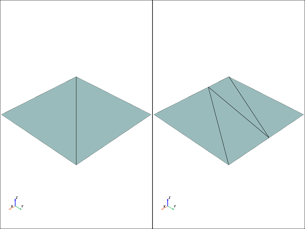
%%px
plot_mesh(serial_mesh)
[output:0]
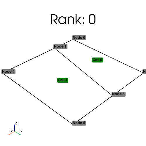
[output:1]
Mesh-partitioning#
As we have seen above, we can send in data to mesh creation and get either a distributed mesh out, but how does it work? Under the hood, what happens is that DOLFINx calls a graph-partitioning algorithm. This algorithm is supplied from either from PT-Scotch[CP08], ParMETIS[KK96] or KaHIP[SS13], depending on what is available with your installation.
We can list the available partitioners with the following code:
%%px
try:
    from dolfinx.graph import partitioner_scotch

    has_scotch = True
except ImportError:
    has_scotch = False
try:
    from dolfinx.graph import partitioner_kahip

    has_kahip = True
except ImportError:
    has_kahip = False
try:
    from dolfinx.graph import partitioner_parmetis

    has_parmetis = True
except ImportError:
    has_parmetis = False
print(f"{has_scotch=}  {has_kahip=} {has_parmetis=}")
[stdout:1] has_scotch=True has_kahip=True has_parmetis=False
[stdout:0] has_scotch=True has_kahip=True has_parmetis=False
Given any of these partitioners (we will from now on use Scotch), you can send them into create mesh by calling
%%px
assert has_scotch
partitioner = dolfinx.mesh.create_cell_partitioner(partitioner_scotch())
quad_mesh = dolfinx.mesh.create_mesh(
    MPIpx.COMM_WORLD,
    cells=quadrilaterals,
    x=quad_points,
    e=ufl_quad,
    partitioner=partitioner,
)
[output:0]
[output:1]
Custom partitioning#
In some cases, one would like to use a specific partitioning. This might be because one have already partitioned the mesh, and when reading it in, one would like to keep this partitioning. We can achieve this by creating a custom partitioner.
%%px
from dolfinx.mesh import CellType
import numpy.typing as npt


def custom_partitioner(
    comm: MPIpx.Intracomm,
    num_partitions: int,
    cell_types: list[CellType],
    topo: list[npt.NDArray[np.int64]],
):
    """Partition a graph"""
    assert len(cell_types) == 1, "Mixed cell types not supported"
    num_vertices_per_cell = dolfinx.cpp.mesh.cell_num_vertices(cell_types[0])
    assert len(topo[0]) // num_vertices_per_cell == len(quadrilaterals)
    dests = np.full(len(topo[0]) // num_vertices_per_cell, comm.rank, dtype=np.int32)
    return dolfinx.graph.adjacencylist(dests)._cpp_object


custom_mesh = dolfinx.mesh.create_mesh(
    MPIpx.COMM_WORLD,
    cells=quadrilaterals,
    x=quad_points,
    e=ufl_quad,
    partitioner=custom_partitioner,
)
num_cells_local = custom_mesh.topology.index_map(2).size_local
num_cells_global = custom_mesh.topology.index_map(2).size_global
num_ghosts = custom_mesh.topology.index_map(2).num_ghosts
print(
    f"Rank: {MPIpx.COMM_WORLD.rank}: {num_cells_local=} {num_ghosts=} {num_cells_global=} (Num input cells: {quadrilaterals.shape[0]})"
)
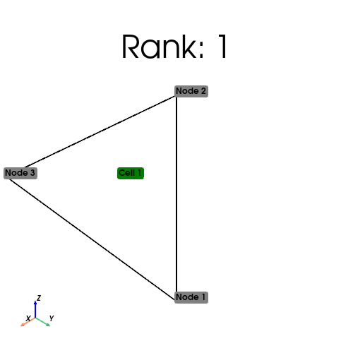
[stdout:0] Rank: 0: num_cells_local=0 num_ghosts=0 num_cells_global=2 (Num input cells: 0)
[stdout:1] Rank: 1: num_cells_local=2 num_ghosts=0 num_cells_global=2 (Num input cells: 2)
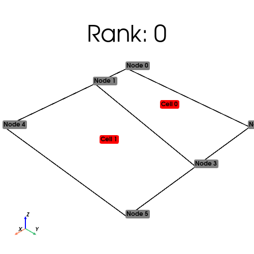
%%px
pyvista.global_theme.allow_empty_mesh = True
plot_mesh(custom_mesh)
[output:1]

Ghosting#
If one wants to use Discontinuous Galerkin methods, one needs extra information in parallel.
To be able to compute interior integrals, every interior facet owned by a process needs to have access to the two cells its connected to.
To be able to control this, one can send in ghost_mode=dolfinx.mesh.GhostMode.shared_facet to the mesh creation algorithm.
We start by inspecting the previously created methods
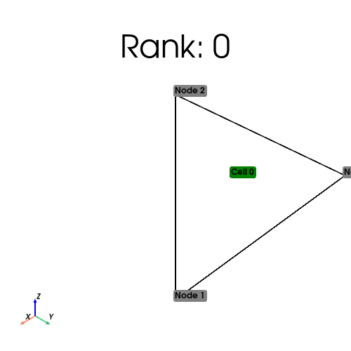
%%px
print(f"Number of ghost cells: {cell_index_map.num_ghosts}")
[stdout:0] Number of ghost cells: 0
[stdout:1] Number of ghost cells: 0
Thus, we observe that we only have cells owned by the process on each rank. By adding ghost mode to the mesh creation:
%%px
shared_partitioner = dolfinx.mesh.create_cell_partitioner(
    dolfinx.mesh.GhostMode.shared_facet
)
ghosted_mesh = dolfinx.mesh.create_mesh(
    MPIpx.COMM_WORLD,
    cells=quadrilaterals,
    x=quad_points,
    e=ufl_quad,
    partitioner=shared_partitioner,
)
num_cells_local = ghosted_mesh.topology.index_map(2).size_local
num_cells_global = ghosted_mesh.topology.index_map(2).size_global
num_ghosts = ghosted_mesh.topology.index_map(2).num_ghosts
print(
    f"Rank: {MPIpx.COMM_WORLD.rank}: {num_cells_local=} {num_ghosts=} {num_cells_global=} (Num input cells: {quadrilaterals.shape[0]})"
)
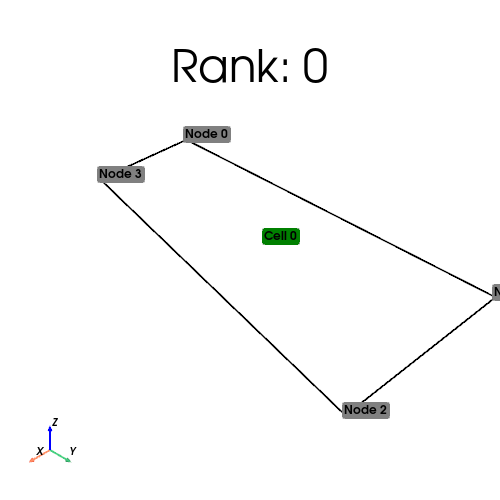
[stdout:1] Rank: 1: num_cells_local=1 num_ghosts=1 num_cells_global=2 (Num input cells: 2)
[stdout:0] Rank: 0: num_cells_local=1 num_ghosts=1 num_cells_global=2 (Num input cells: 0)
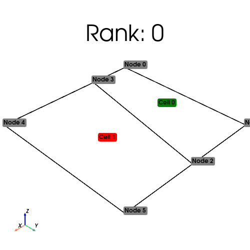
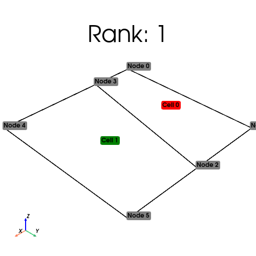
We visualize the owned cells in green, and the ghosted cells in red below
%%px
pyvista.global_theme.allow_empty_mesh = True
plot_mesh(ghosted_mesh, include_ghosts=True)
[output:0]
[output:1]
We can also add ghosting to the partitioning routine. Let’s say that we want to assign the cells on process 0 to process 1, but keep them as ghosts on process 0, then a custom partitioning could look like
%%px


def custom_ghosted_partitioner(
    comm: MPIpx.Intracomm,
    num_partitions: int,
    cell_types: list[CellType],
    topo: list[npt.NDArray[np.int64]],
):
    """Partition a graph"""
    assert len(cell_types) == 1, "Mixed cell types not supported"
    num_vertices_per_cell = dolfinx.cpp.mesh.cell_num_vertices(cell_types[0])
    assert len(topo[0]) // num_vertices_per_cell == len(quadrilaterals)
    if len(topo[0]) > 0:
        dests = np.empty(
            (len(topo[0]) // num_vertices_per_cell, comm.size), dtype=np.int32
        )
        all_ranks = np.arange(comm.size, dtype=np.int32)
        all_ranks = np.delete(all_ranks, 1)
        dests[:, 0] = 1  # Rank that should own this cell is assigned first.
        dests[:, 1:] = (
            all_ranks  # Assign all cells on process as ghosts on all but process 1
        )
    else:
        dests = np.empty(0, dtype=np.int32)
    adj = dolfinx.graph.adjacencylist(dests)
    print(comm.rank, comm.size, adj._cpp_object)
    return adj._cpp_object


ghosted_custom_mesh = dolfinx.mesh.create_mesh(
    MPIpx.COMM_WORLD,
    cells=quadrilaterals,
    x=quad_points,
    e=ufl_quad,
    partitioner=custom_ghosted_partitioner,
)


num_cells_local = ghosted_custom_mesh.topology.index_map(2).size_local
num_cells_global = ghosted_custom_mesh.topology.index_map(2).size_global
num_ghosts = ghosted_custom_mesh.topology.index_map(2).num_ghosts
print(
    f"Rank: {MPIpx.COMM_WORLD.rank}: {num_cells_local=} {num_ghosts=} {num_cells_global=} (Num input cells: {quadrilaterals.shape[0]})"
)
[stdout:0] 0 2 <AdjacencyList> with 0 nodes

Rank: 0: num_cells_local=0 num_ghosts=2 num_cells_global=2 (Num input cells: 0)
[stdout:1] 1 2 <AdjacencyList> with 2 nodes
  0: [1 0 ]
  1: [1 0 ]

Rank: 1: num_cells_local=2 num_ghosts=0 num_cells_global=2 (Num input cells: 2)
%%px
pyvista.global_theme.allow_empty_mesh = True
plot_mesh(ghosted_custom_mesh, include_ghosts=True)
[output:1]
[output:0]
References#
C. Chevalier and F. Pellegrini. Pt-scotch: a tool for efficient parallel graph ordering. Parallel Computing, 34(6):318–331, 2008. Parallel Matrix Algorithms and Applications. doi:10.1016/j.parco.2007.12.001.
George Karypis and Vipin Kumar. Parallel multilevel k-way partitioning scheme for irregular graphs. In Proceedings of the 1996 ACM/IEEE Conference on Supercomputing, Supercomputing '96, 35–es. USA, 1996. IEEE Computer Society. doi:10.1145/369028.369103.
Peter Sanders and Christian Schulz. Think locally, act globally: highly balanced graph partitioning. In Vincenzo Bonifaci, Camil Demetrescu, and Alberto Marchetti-Spaccamela, editors, Experimental Algorithms, 164–175. Berlin, Heidelberg, 2013. Springer Berlin Heidelberg. doi:10.1007/978-3-642-38527-8_16.
Matthew W. Scroggs, Jørgen S. Dokken, Chris N. Richardson, and Garth N. Wells. Construction of arbitrary order finite element degree-of-freedom maps on polygonal and polyhedral cell meshes. ACM Trans. Math. Softw., May 2022. doi:10.1145/3524456.