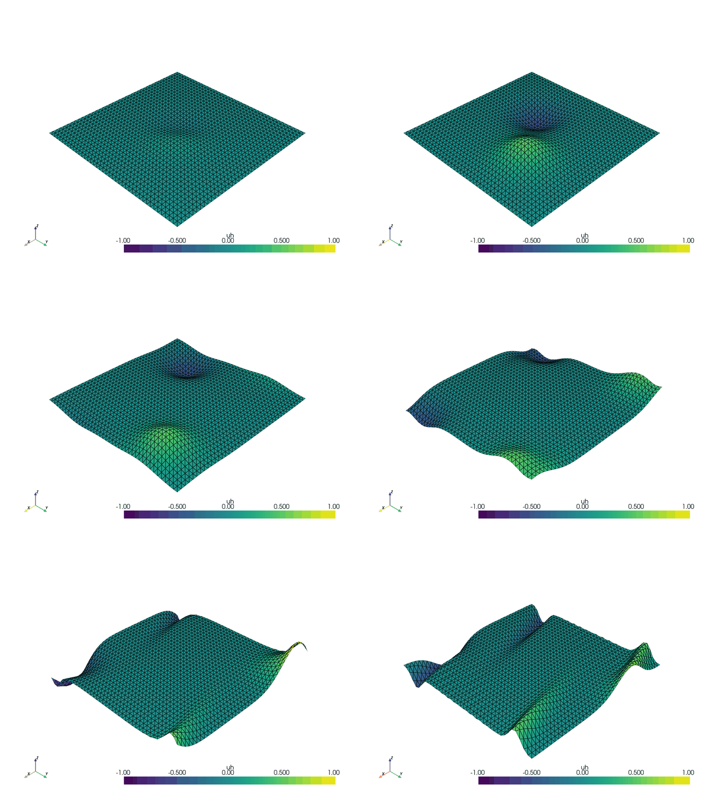
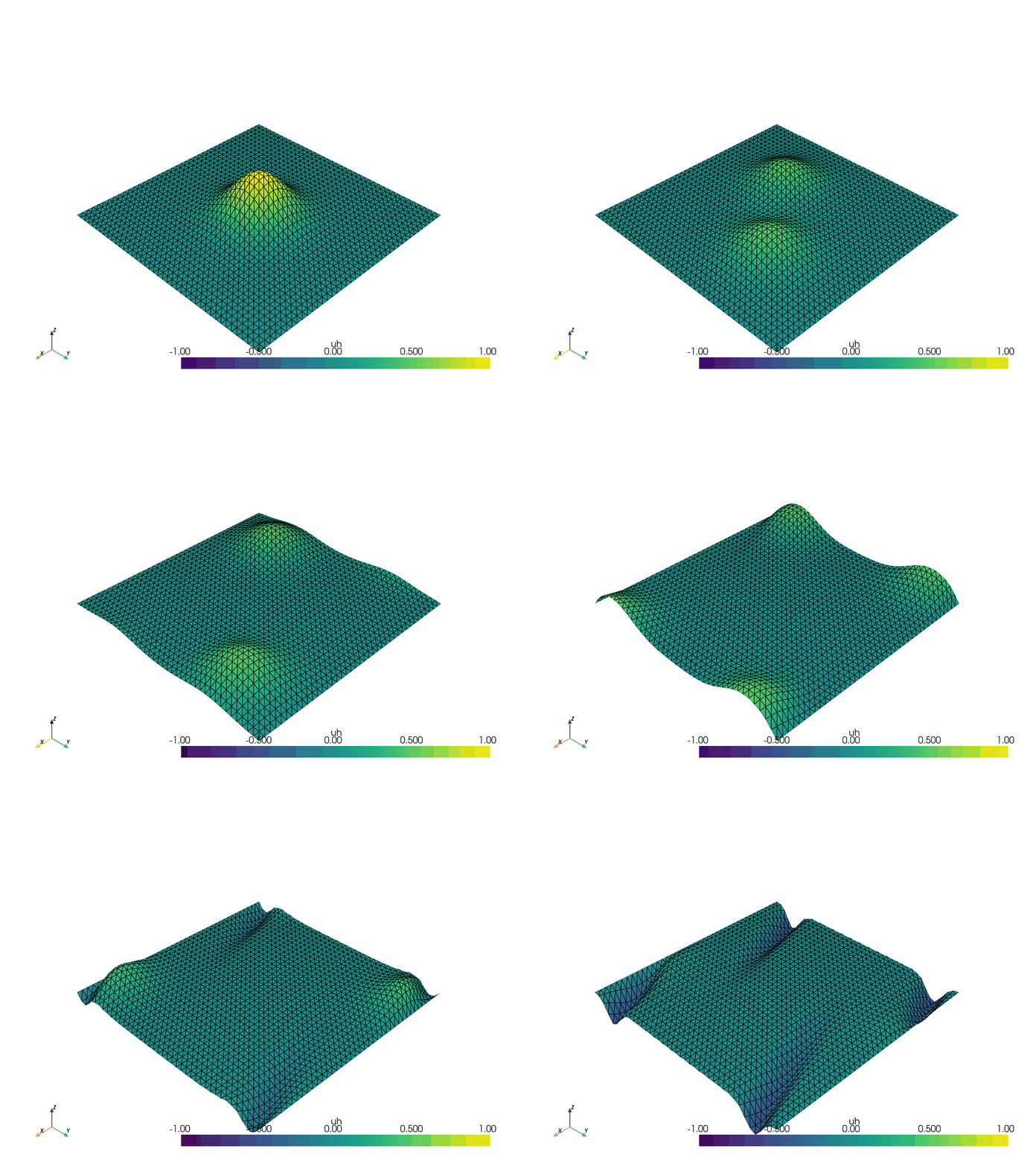
Anisotropic wave system with periodic boundary conditions

Author Jørgen S. Dokken and Markus Renoldner

License MIT

This demo illustrates how to use the MPC package to enforce periodic boundary conditions for a linear wave problem.

Mathematical formulation

We want to compute two time-dependent functions \((u,\phi)\) on the unitsquare \(\Omega=(0,1)^2\), that solve

\[\begin{split} \begin{cases} \displaystyle \partial_{t} u + b\cdot \nabla \phi=0, \\ \partial_{t} \phi + b\cdot \nabla u=0, \end{cases} \end{split}\]

where the given vectorfield satisfies \((\operatorname{div} b = 0)\), that dictates the advection direction, and \((f,g)\) are given functions.

Smooth solutions of the above system also satisfy a decoupled version of the above system,

\[ \partial_{tt} u + b\cdot\nabla (b\cdot\nabla u) = 0. \]

This last problem resembles the linear wave equation, which explains the wavey dynamics of the solution.

The aim of this tutorial is to show how to use periodic boundary conditions. We will choose the following setting:

\[\begin{split} \begin{align*} \phi|_{\Gamma_D} &=0 , \\ \phi|_{\Gamma_l} &= \phi|_{\Gamma_r}, \\ u|_{\Gamma_l} &= |_{\Gamma_r}, \end{align*} \end{split}\]

where we set \((\partial\Omega = \Gamma_D\cup \Gamma_l \cup \Gamma_r)\), with

\[\begin{split} \begin{align*} \Gamma_D &:=\{(x,y)\in \bar{\Omega}: y=0 \text{ or }y=1\},\quad&&\text{i.e. the bottom and top wall}\\ \Gamma_l &:=\{(x,y)\in \bar{\Omega}: x=0\},\quad&&\text{i.e. the left wall}\\ \Gamma_r &:=\{(x,y)\in \bar{\Omega}: x=1\},\quad&&\text{i.e. the right wall}. \end{align*} \end{split}\]

We start by the various modules required for this demo

import typing
from pathlib import Path

from mpi4py import MPI
from petsc4py import PETSc

import dolfinx.fem as fem
import dolfinx.la.petsc
import numpy as np
import pyvista
from basix.ufl import element
from dolfinx import default_real_type, default_scalar_type, plot
from dolfinx.fem import Constant, Function, assemble_scalar, form, functionspace
from dolfinx.mesh import create_unit_square, locate_entities_boundary
from ufl import (
    FacetNormal,
    MixedFunctionSpace,
    SpatialCoordinate,
    TestFunctions,
    TrialFunctions,
    dx,
    extract_blocks,
    grad,
    inner,
)

from dolfinx_mpc import (
    MultiPointConstraint,
    apply_lifting,
    assemble_matrix,
    assemble_vector,
    create_vector,
)

Next, we create some convenience functions to create a gif from a given function.

Each process builds a PyVista grid over the cells it owns, so a shared cell is not drawn twice, and the grids are gathered onto one process which draws them into a single figure and writes a single GIF, with common colour limits.

The geometry does not move, so the grids are gathered once when the animation is opened and only the nodal values are communicated per frame.

pyvista.global_theme.allow_empty_mesh = True


class GatheredGrid(typing.NamedTuple):
    """Owned-cell PyVista grids of a distributed function, gathered on one process."""

    comm: MPI.Comm
    root: int
    num_points: int
    pieces: typing.Optional[list[pyvista.UnstructuredGrid]]

    @classmethod
    def create(cls, V: fem.FunctionSpace, root: int = 0) -> "GatheredGrid":
        """Gather the geometry, which does not change, once.

        ``root`` is kept on the object so that the values gathered later cannot
        end up on a different process than the grids they belong to.
        """
        tdim = V.mesh.topology.dim
        owned_cells = np.arange(V.mesh.topology.index_map(tdim).size_local, dtype=np.int32)
        grid = pyvista.UnstructuredGrid(*plot.vtk_mesh(V, entities=owned_cells))
        comm = V.mesh.comm
        return cls(comm, root, grid.n_points, comm.gather(grid, root=root))

    @property
    def is_root(self) -> bool:
        """Whether this process is the one holding the gathered grids."""
        return self.comm.rank == self.root

    def gather_values(self, plotfunc: fem.Function) -> typing.Optional[list[np.ndarray]]:
        """Collect the nodal values of each partition on the root process.

        ``plotfunc`` may live in the constraint's extended space, whose array is
        longer than the original space; the extended index map keeps the original
        dofs first, so the leading entries are the ones the grid refers to.
        """
        return self.comm.gather(plotfunc.x.array.real[: self.num_points].copy(), root=self.root)


def create_gif(
    plotfunc: fem.Function, filename: Path, fps: float, root: int = 0
) -> tuple[GatheredGrid, typing.Optional[pyvista.Plotter]]:
    """
    Create a GIF animation from a given plotting function and function space.

    Args:
        plotfunc: The plotting function that generates the data to be visualized.
        filename: The name of the output GIF file.
        fps: Frames per second for the GIF animation.
        root: The process that gathers the pieces and writes the animation.
    Returns:
        tuple: The gathered grid, and the plotter on ``root`` (``None`` elsewhere).

    Example:

        .. code-block:: python

            grid, plotter = create_gif(plotfunc, Path("output.gif"), 10)

            for i in range(N):
                plotter = update_gif(...)
            finalize_gif(...)
    """
    grid = GatheredGrid.create(plotfunc.function_space, root=root)
    plotter = None
    if grid.is_root:
        plotter = pyvista.Plotter(off_screen=True)
        plotter.open_gif(filename, fps=fps)
        plotter.show_axes()  # type: ignore[call-arg]
    return grid, plotter


def update_gif(
    grid: GatheredGrid,
    plotter: pyvista.Plotter | None,
    plotfunc: fem.Function,
    warp_gif: bool,
    clip_gif: bool,
    clip_normal: typing.Literal["x", "y", "z", "-x", "-y", "-z"] = "y",
) -> pyvista.Plotter | None:
    """
    Add one frame, drawing every partition of the solution into a single figure.

    Args:
        grid: The gathered grid to be plotted.
        plotter: The plotter instance used for plotting, on the root process.
        plotfunc: An object containing the data to be plotted, with an attribute `x.array`.
        warp_gif: If True, warp the grid by the scalar values.
        clip_gif: If True, clip the grid along the specified normal.
        clip_normal: The normal direction for clipping. Default is "y".

    Returns:
        The updated plotter instance on the root process, and None elsewhere.
        The root is the one given to :func:`create_gif`, and is carried on ``grid``.
    """
    # Collective: every process contributes its piece
    values = grid.gather_values(plotfunc)
    if not grid.is_root:
        return plotter
    assert plotter is not None and grid.pieces is not None and values is not None

    # A fixed range keeps the colours comparable between frames and partitions
    maxval = 1.0
    plotter.clear()
    if warp_gif and clip_gif:
        PETSc.Sys.Print("warp and clip not possible at the same time")  # type: ignore
    for piece, piece_values in zip(grid.pieces, values):
        piece.point_data["uh"] = piece_values
        if warp_gif and not clip_gif:
            plotter.add_mesh(
                piece.warp_by_scalar("uh", factor=0.2 / maxval),
                clim=[-maxval, maxval],
                show_edges=True,
            )
        elif clip_gif:
            plotter.add_mesh(piece.clip(clip_normal, invert=True), clim=[-maxval, maxval], show_edges=True)
            plotter.add_mesh(piece, style="wireframe", clim=[-maxval, maxval], show_edges=True)
        else:
            plotter.add_mesh(piece, clim=[-maxval, maxval], show_edges=True)

    plotter.write_frame()
    plotter.show_axes()  # type: ignore[call-arg]
    return plotter


def finalize_gif(plotter: typing.Optional[pyvista.Plotter]):
    if plotter is not None:
        plotter.close()

The goal is to solve the wave system using Lagrange Finite Elements. For this we propose the following weak formulation:

\[\begin{split} \begin{cases} \displaystyle \int_\Omega \partial_{t}u v + \int_\Omega b\cdot\nabla\phi v=0 \quad \forall v \in X^r(\Omega)\\ \displaystyle\int_\Omega \partial_{t} \phi \psi - \int_\Omega u b\cdot\nabla\psi = 0 \quad \forall \psi\in X^r_0(\Omega) \end{cases} \end{split}\]

Here \((X^r)\) denotes the Lagrange order \((r)\), global FEM space of piecewise polynomial functions that are globally continuous, defined as

\[ X^r(\Omega) := \{u_h \in C (\bar{\Omega} ) : u_h |_K \in \mathbb{P}^r\ \forall K\} . \]

The notation \((X^r_0)\) denotes the restriction of the above space to a space with zero boundary values.

For the derivative in time, we use the Crank-Nicolson scheme. We define some matrices:

\[\begin{split} \begin{aligned} M_{ij} &= \left \langle v_j, v_i \right \rangle \\ N_{ij} &= \left \langle \psi_j,\psi_i \right \rangle \\ E_{ij} &= \left \langle \nabla\psi_j , b v_i \right \rangle \\ F_{ij} &= \left \langle v_j b,\nabla \psi_i\right \rangle \end{aligned} \end{split}\]

The scheme is then:

\[\begin{split} \begin{aligned} \begin{pmatrix} M & + \frac{\Delta t}{2}E \\ - \frac{\Delta t}{2}F & N \end{pmatrix} \begin{pmatrix} \vec u ^{n+1}\\ \vec\phi^{n+1} \end{pmatrix} = \begin{pmatrix} M \vec u^n - \frac{\Delta t}{2} E \vec\phi^n\\ \frac{\Delta t}{2} F\vec u^n +N\vec \phi^n \end{pmatrix} \end{aligned} \end{split}\]

It turns out the continuous problem, as well as the fully discrete version is stable, and one can show, that solutions \((u,\phi)\) conserve the energy

\[\mathcal{E} := \int_\Omega u^2 +\phi^2.\]

We will now implement this problem in fenicsx.

dt = 0.02  # time step
t = 0.0  # initial time
T_end = 1  # final time
num_steps = int(T_end / dt)  # number of time steps
Nx = 40  # number of elements in x and y direction
h = 1 / Nx  # mesh size
bconst = 1.0  # magnitude of the advection field

# A single animation is written however many processes are used
# The GIF of the pressure, shown in the gallery of the documentation, is named after the demo
figure = Path("demo_linear_wave_problem.py")
filename_gifV = figure.with_name(f"{figure.stem}_velocity.gif")
filename_gifp = figure.with_suffix(".gif")

warp_gif = True

Mesh, spaces, functions

We create a ufl.MixedFunctionSpace for the functions V,p

msh = create_unit_square(MPI.COMM_WORLD, Nx, Nx, dtype=default_real_type)
P1 = element("Lagrange", "triangle", 1, dtype=default_real_type)
XV = functionspace(msh, P1)
Xp = functionspace(msh, P1)
Z = MixedFunctionSpace(XV, Xp)
eps = 0.8
bfield = Constant(msh, default_scalar_type(((eps), np.sqrt(1 - eps**2))))
x = SpatialCoordinate(msh)
n = FacetNormal(msh)

Dirichlet BC Along the top and bottom wall, we set `p=0``

facets = locate_entities_boundary(
    msh, dim=1, marker=lambda x: np.logical_or.reduce((np.isclose(x[1], 1.0), np.isclose(x[1], 0.0)))
)
dofs = fem.locate_dofs_topological(V=Xp, entity_dim=1, entities=facets)
bcs = [fem.dirichletbc(np.array(0.0, dtype=default_scalar_type), dofs=dofs, V=Xp)]

Periodic BC

Along the left and right wall, we set periodic boundary conditions

tol = 250 * np.finfo(default_scalar_type).resolution

We will now identify the set \(\{(x,y) \in \partial \Omega: x=1\}\)

def periodic_boundary(x):
    return np.isclose(x[0], 1, atol=tol)

Now we define the periodic identification of points on the left and right wall This identification is only valid on the periodic boundary

def periodic_relation(x):
    out_x = np.zeros_like(x)
    out_x[0] = 0  # map x=1 to x=0
    out_x[1] = x[1]  # keep y-coord as is
    return out_x

For each of the sapces Xp, XV, we create a dolfinx_mpc.MultiPointConstraint and use create_periodic_constraint_geometrical to create the periodic constraints

mpc_p = MultiPointConstraint(Xp)
mpc_p.create_periodic_constraint_geometrical(Xp, periodic_boundary, periodic_relation, bcs)
mpc_p.finalize()

mpc_V = MultiPointConstraint(XV)
mpc_V.create_periodic_constraint_geometrical(XV, periodic_boundary, periodic_relation, bcs)
mpc_V.finalize()

We can now define the dolfinx.fem.Function for the new time step values, as well as the trial and test functions

Note

Note that we use the mpc.function_space as input for the functions.

# new time step values
V_new = fem.Function(mpc_V.function_space, dtype=default_scalar_type)
p_new = fem.Function(mpc_p.function_space, dtype=default_scalar_type)
V, p = TrialFunctions(Z)
W, q = TestFunctions(Z)

# initial conditions
V_old = Function(mpc_V.function_space, dtype=default_scalar_type)
p_old = Function(mpc_p.function_space, dtype=default_scalar_type)
V_old.interpolate(lambda x: 0.0 * x[0])
p_old.interpolate(lambda x: np.exp(-1 * (((x[0] - 0.5) / 0.15) ** 2 + ((x[1] - 0.5) / 0.15) ** 2)))

We set up the gifs using the convenience function defined above

gridV, plotterV = create_gif(V_old, filename_gifV, fps=0.1 / dt)
gridp, plotterp = create_gif(p_old, filename_gifp, fps=0.1 / dt)

We define the weak form of the left hand side and use extract_blocks to extract the block structure of the bilinear form.

M = inner(V, W) * dx
E = inner(grad(p), bfield * W) * dx
F = inner(grad(V), bfield * q) * dx
N = inner(p, q) * dx
a = M + dt / 2 * E + dt / 2 * F + N
a_blocked = form(extract_blocks(a), dtype=default_scalar_type)

As the system matrix is time-independent, we use assemble_matrix with kind="nest" to create and assemble the system matrix once, outside the temporal loop.

A = assemble_matrix(a_blocked, [mpc_V, mpc_p], bcs, kind="nest")

We define the Krylov subspace solver using petsc4py.PETSc.KSP and use a direct LU solver as preconditioner.

solver = PETSc.KSP().create(msh.comm)  # type: ignore
solver.setOperators(A)
solver.setType(PETSc.KSP.Type.PREONLY)  # type: ignore
solver.getPC().setType(PETSc.PC.Type.LU)  # type: ignore

As we did for the bilinear form, we define the linear form, extract the block structure, and create the petsc4py.PETSc.Vec that we will assemble into at each time step.

L = (
    inner(V_old, W) * dx
    - dt / 2 * inner(grad(p_old), bfield * W) * dx
    + inner(p_old, q) * dx
    - dt / 2 * inner(grad(V_old), bfield * q) * dx
)
L_blocked = form(extract_blocks(L), dtype=default_scalar_type)
b = create_vector(L_blocked, [mpc_V, mpc_p], kind="nest")

We perform the time dependent solve in a temporal loop. Note that we use assemble_vector, apply_lifting, and backsubstitution to handle the periodic conditions.

Note

Assembly is additive, as in DOLFINx, so the vector has to be zeroed before it is reassembled at each time step. Without it the right hand side accumulates the contributions of all previous steps, and the solution grows exponentially.

def energy(V_h, p_h):
    """The squared L2 norm of the solution, summed over the processes."""
    local = assemble_scalar(form(inner(V_h, V_h) * dx + inner(p_h, p_h) * dx))
    return msh.comm.allreduce(local, op=MPI.SUM).real


progress_0 = 0
for i in range(num_steps):
    t += dt

    # update RHS
    dolfinx.la.petsc._zero_vector(b)
    assemble_vector(L_blocked, [mpc_V, mpc_p], b)

    # Dirichlet BC values in RHS
    apply_lifting(b, a_blocked, bcs, [mpc_V, mpc_p])
    dolfinx.la.petsc._ghost_update(
        b,
        insert_mode=PETSc.InsertMode.ADD_VALUES,  # type: ignore
        scatter_mode=PETSc.ScatterMode.REVERSE,  # type: ignore
    )
    bcs0 = fem.bcs_by_block(fem.extract_function_spaces(L_blocked), bcs)
    fem.petsc.set_bc(b, bcs0)

    # solve
    Vp_vec = b.copy()
    solver.solve(b, Vp_vec)
    dolfinx.la.petsc._ghost_update(
        Vp_vec,
        insert_mode=PETSc.InsertMode.INSERT,  # type: ignore
        scatter_mode=PETSc.ScatterMode.FORWARD,  # type: ignore
    )  # type: ignore
    dolfinx.fem.petsc.assign(Vp_vec, [V_new, p_new])

    # update MPC slave dofs
    mpc_V.backsubstitution(V_new)
    mpc_p.backsubstitution(p_new)

    # The initial condition is only periodic up to the tails of the Gaussian, so the energy is
    # compared with that of the first step, whose values are constrained
    if i == 0:
        E_reference = energy(V_new, p_new)

    # progress
    progress = int(((i + 1) / num_steps) * 100)
    if progress >= progress_0 + 20:
        progress_0 = progress
        PETSc.Sys.Print(f"|--progress: {progress}% \t time: {t:6.5f} \t E={energy(V_new, p_new):.15e}:")  # type: ignore

    # Update solution at previous time step
    V_old.x.array[:] = V_new.x.array
    p_old.x.array[:] = p_new.x.array

    # gif
    plotterV = update_gif(gridV, plotterV, V_old, warp_gif, clip_gif=False)
    plotterp = update_gif(gridp, plotterp, p_old, warp_gif, clip_gif=False)

solver.destroy()
b.destroy()
Vp_vec.destroy()

|--progress: 20% 	 time: 0.20000 	 E=3.501905082164685e-02:

|--progress: 40% 	 time: 0.40000 	 E=3.501905082164704e-02:

|--progress: 60% 	 time: 0.60000 	 E=3.501905082164707e-02:

|--progress: 80% 	 time: 0.80000 	 E=3.501905082164693e-02:

|--progress: 100% 	 time: 1.00000 	 E=3.501905082164709e-02:

<petsc4py.PETSc.Vec at 0x7f3956e14770>

The Crank-Nicolson scheme conserves the energy \(\|u\|^2+\|\phi\|^2\) of this skew-symmetric system, which verifies the solution.

assert abs(energy(V_old, p_old) - E_reference) < 1e4 * np.finfo(default_real_type).eps * E_reference

We store the GIF to file

finalize_gif(plotterV)
finalize_gif(plotterp)
PETSc.Sys.Print(f"gifs saved as {filename_gifV}, {filename_gifp}")  # type: ignore

gifs saved as demo_linear_wave_problem_velocity.gif, demo_linear_wave_problem.gif