A double pendulum: two beams on two pins#
Author Jørgen S. Dokken
License MIT
In this demo we will explore coupling two separately meshes elastic beams that are coupled to each other through a stiff spring, forming a double pendulum. Beam 1 turns about a fixed pin through a bore at its top. A second pin, through a bore lower down in beam 1, carries beam 2, which hangs beside beam 1 and turns about that pin. All the pins are created by using RBE2 spiders, as in Joining two bodies with a rigid spider (RBE2), and the two spiders of the lower pin are coupled by a stiff spring. We start by importing the required dependencies:
The beams#
Two beams hang from two pins that run along \(y\); gravity points along \(-z\). Each beam is a box of depth \(H\) along \(x\), centred on \(x = 0\), with a bore of radius \(r\) around each pin it hangs on or carries:
Beam 1, of width \(W_0\) along the pins, \(y \in [0, W_0]\), hangs from the fixed pin at height \(z = 0\) and reaches down to \(z = -L\). A second bore, for the lower pin, is at \(z = -0.8 L\).
Beam 2, of width \(W_1\), hangs beside beam 1, a gap \(s\) away along the pins, \(y \in [W_0 + s, W_0 + s + W_1]\), from a bore on the lower pin, and reaches a length \(L_2\) below it.
Above its top bore, each beam has a margin \(e = 2.5 r\) of material. On the axis of each pin, at the middle of each beam’s bore, the points \(x_P\), \(x_A\) and \(x_B\) are the spiders of the next section.
comm = MPI.COMM_WORLD
L, W_0, H = 2.0, 0.4, 0.3  # Beam 1: length below its top bore, width along the pins, depth
L_2, W_1 = 1.5, 0.25  # Beam 2: length below its bore, width along the pins
radius, gap = 0.08, 0.05  # The bores' radius, and the gap between the beams along the pins
margin = 2.5 * radius  # The material above a beam's top bore
z_top, z_pin = 0.0, -0.8 * L  # The heights of the fixed pin and of the lower pin

# Each beam's extent along the pins (y) and along gravity (z), and the heights of its bores
beam_1_y, beam_1_z, beam_1_bores = (0.0, W_0), (-L, z_top + margin), [z_top, z_pin]
beam_2_y, beam_2_z, beam_2_bores = (W_0 + gap, W_0 + gap + W_1), (z_pin - L_2, z_pin + margin), [z_pin]

# The spiders, on the pins' axes at x = 0, at the middle of each bore along the pin
x_P = np.array([0.0, 0.5 * sum(beam_1_y), z_top], dtype=default_real_type)
x_A = np.array([0.0, 0.5 * sum(beam_1_y), z_pin], dtype=default_real_type)
x_B = np.array([0.0, 0.5 * sum(beam_2_y), z_pin], dtype=default_real_type)
The spiders#
The pins are rigid, and they are not part of the simulation mesh: neither the pins nor anything inside the bores is meshed. Instead, the surface of each bore is tied rigidly to a spider (RBE2, as in Joining two bodies with a rigid spider (RBE2)), so that the bore keeps its shape and moves as one rigid body with its spider. The spiders are the points \(x_P\), \(x_A\) and \(x_B\) defined above, on the pins’ axes at the middle of each bore: \(x_P\) in beam 1’s upper bore, and \(x_A\) and \(x_B\) in the lower bores of beam 1 and beam 2, so that \(d = x_B - x_A\) runs along the lower pin. Each spider has six unknowns, its translation \(t\) and its rotation \(\theta\).
The fixed pin lets beam 1 turn about it, but not move: the translation of spider P is pinned, \(t_P = 0\), by Dirichlet conditions on its translation dofs. Its rotations about \(x\) and \(z\) are pinned as well, as a pin through a bore holds them too, so only the rotation about the pin, \(\theta_P \cdot a\) with \(a = (0, 1, 0)\), is free.
The lower pin lets beam 2 turn about it, relative to beam 1, and holds every other relative motion. Beam 1 and beam 2 each have their own spider on it, A and B, joined by a 0-D spring that is stiff in every direction except rotation about the pin.
Each spider is the only point of its own spider mesh, made by
create_spider_mesh, and
create_spider_pair relates spider A to
spider B, for the spring.
spiders_P, spiders_A, spiders_B = (dolfinx_mpc.create_spider_mesh(comm, x.reshape(1, 3)) for x in (x_P, x_A, x_B))
pair = dolfinx_mpc.create_spider_pair(spiders_A, spiders_B)
Next, we create the function spaces on the spider meshes, which should have six components, three for translation and three for rotation.
element = basix.ufl.element("DG", "point", 0, shape=(6,), dtype=default_real_type)
W_P, W_A, W_B = (fem.functionspace(spiders, element) for spiders in (spiders_P, spiders_A, spiders_B))
Meshing the two beams with bores#
Each beam is meshed separately from its extent and the heights of its bores, above, with second order cells: beam 1 with tetrahedra, beam 2 with hexahedra, by extruding a quadrilateral mesh of its side along the pin. The facets of bore \(k\) are tagged \(k + 1\).
beam_1, tags_1 = beam(*beam_1_z, *beam_1_y, beam_1_bores, 0.08, "beam_1")
beam_2, tags_2 = beam(*beam_2_z, *beam_2_y, beam_2_bores, 0.05, "beam_2", hexahedra=True)
The meshes of the beams, and the spider nodes as spheres, taken from the spider meshes. Each process makes a grid of the cells it owns, from the geometry of the mesh alone, and the pieces are gathered on one process. The cells are drawn curved, as the mesh’s second order cells, with the edges of the first order cells through their vertices. In the collapsed section below you will find some utlities for plotting the meshes with pyvista.
The constraints#
Both beams are discretized in the same way: the displacement of each is in a space of
second order vector Lagrange elements on its second order mesh, of tetrahedra and of
hexahedra respectively.
The upper bore of beam 1 follows spider P, its lower bore spider A, and the bore of
beam 2 spider B. Spiders A and B have no constraint of their own, and we therefore create
empty MultiPointConstraints for them.
The pinned dofs of spider P, its translation and its rotations about \(x\) and \(z\), are masters of the upper bore. Their Dirichlet conditions are therefore given to spider P’s constraint, which removes them from the bore’s relation, as well as to the problems below, which set them.
V_1 = fem.functionspace(beam_1, ("Lagrange", 2, (3,)))
V_2 = fem.functionspace(beam_2, ("Lagrange", 2, (3,)))

mpc_1 = dolfinx_mpc.MultiPointConstraint(V_1, dtype=default_scalar_type)
mpc_1.add_rbe2_topological(2, tags_1.find(1), W_P)
mpc_1.add_rbe2_topological(2, tags_1.find(2), W_A)

mpc_2 = dolfinx_mpc.MultiPointConstraint(V_2, dtype=default_scalar_type)
mpc_2.add_rbe2_topological(2, tags_2.find(1), W_B)
# The translation (0, 1, 2) and the rotations about x and z (3, 5) of spider P
cells_P = np.arange(spiders_P.topology.index_map(0).size_local, dtype=np.int32)
zero = default_scalar_type(0.0)
pinned = [
    fem.dirichletbc(zero, fem.locate_dofs_topological(W_P.sub(i), 0, cells_P), W_P.sub(i)) for i in (0, 1, 2, 3, 5)
]
mpc_P = dolfinx_mpc.MultiPointConstraint(W_P, dtype=default_scalar_type, bcs=pinned)
mpcs = [mpc_1, mpc_2, mpc_P] + [dolfinx_mpc.MultiPointConstraint(V, dtype=default_scalar_type) for V in (W_A, W_B)]

dolfinx_mpc.finalize_multipointconstraints(mpcs)
The spring coupling#
With \(w = (t, \theta)\) the translation and rotation of a spider, the two spiders of the lower pin, at \(x_A\) in beam 1 and \(x_B\) in beam 2, are held together if spider B moves as a rigid extension of spider A, \(t_B = t_A + \theta_A \times d\) with \(d = x_B - x_A\), and \(\theta_B = \theta_A\). The spring stores the energy \(\frac12 \delta \cdot K \delta\), with
with \(a\) the direction of the pin, \(k\) large, and \(k_t\) the stiffness against turning about the pin, zero for a free pin. The fixed pin is held by its Dirichlet conditions, so its spring only acts against turning, \(K_P = k_t\, a a^T\) on the rotation of spider P. The springs involve only the spiders. With \(w = (w_P, w_A, w_B)\) the unknowns of the three spiders and \(z = (z_P, z_A, z_B)\) their test functions, the springs of both pins form the bilinear form
the first integrated over spider mesh A, reaching spider B through the pair, the second
over spider mesh P. The function springs(K_pins, w, z) builds it for given stiffnesses. Both
springs are locked, \(k_t = k\), for the static deflection, and free, \(k_t = 0\), for the
swing, the two stages of the solution below.
axis = np.array([0.0, 1.0, 0.0])
d = fem.Constant(spiders_A, (x_B - x_A).astype(default_scalar_type))


def spring_gap(w_A, w_B):
    """The motion of spider B away from the rigid extension of spider A."""
    t_A, theta_A = ufl.as_vector([w_A[i] for i in range(3)]), ufl.as_vector([w_A[i] for i in range(3, 6)])
    t_B, theta_B = ufl.as_vector([w_B[i] for i in range(3)]), ufl.as_vector([w_B[i] for i in range(3, 6)])
    translation = t_B - t_A - ufl.cross(theta_A, d)
    rotation = theta_B - theta_A
    return ufl.as_vector([translation[i] for i in range(3)] + [rotation[i] for i in range(3)])


def spring_stiffness(k_t: float) -> np.ndarray:
    """The 6x6 stiffness of the spring, with `k_t` against turning about the pin."""
    K = np.zeros((6, 6))
    K[:3, :3] = k * np.eye(3)
    K[3:, 3:] = k * (np.eye(3) - np.outer(axis, axis)) + k_t * np.outer(axis, axis)
    return K.astype(default_scalar_type)


def torsion(k_t: float) -> np.ndarray:
    """The 6x6 stiffness of the fixed pin against turning about it, its other dofs being pinned."""
    K_P = np.zeros((6, 6))
    K_P[3:, 3:] = k_t * np.outer(axis, axis)
    return K_P.astype(default_scalar_type)


def springs(K_pins, w, z):
    """The springs of both pins, s(w, z), with the stiffnesses `K_pins`, for the spider parts
    `w = (w_P, w_A, w_B)` and `z` of the unknowns and the test functions."""
    (w_P, w_A, w_B), (z_P, z_A, z_B) = w, z
    lower = ufl.inner(K_pins[0] * spring_gap(w_A, w_B), spring_gap(z_A, z_B)) * ufl.dx(spiders_A)
    return lower + ufl.inner(K_pins[1] * w_P, z_P) * ufl.dx(spiders_P)
The variational problem#
The motion of the system follows from its energies. With the unknowns \(u = (u_1, u_2, w)\) of the whole system, the displacements \(u_b\) of the beams \(\Omega_b\), \(b = 1, 2\), and the spiders’ \(w = (w_P, w_A, w_B)\), the kinetic energy is \(\frac12 M(\dot u, \dot u)\) and the potential energy is
with \(W_b\) the strain energy density of beam \(b\), of Lamé parameters \(\mu_b\) and \(\lambda_b\) from its Young’s modulus \(E_b\) and Poisson’s ratio \(\nu_b\), \(\mathcal{E}\) the Green–Lagrange strain, \(F\) the work of gravity \(g\), and \(s\) the springs of The spring coupling, above. Here
with \(\rho_b\) the density of beam \(b\). By Hamilton’s principle, the motion makes \(\int \left(\frac12 M(\dot u, \dot u) - \Pi(u)\right)~\mathrm{d}t\) stationary.
The meshes are the reference configuration: the beams as built, before gravity acts. We decompose the displacement from it into two parts, \(u_0 + u\):
\(u_0\), the static deflection under gravity, which brings the beams to the hanging state, at rest;
\(u\), the small motion about the hanging state: the swing.
Both follow from \(\Pi\). As \(u_0\) is small, both are computed on the reference configuration, and the animation below shows the swing \(u\).
\(M\), \(a\), \(a_{\sigma_0}\) and \(F\), below, involve only the beams, and \(s\) only the spiders.
The hanging state#
The deflection \(u_0 = (u_{0,1}, u_{0,2}, w_0)\) minimizes \(\Pi\). It is small, so \(\mathcal{E} \approx \varepsilon\), and the minimum satisfies
for all test functions \(v = (v_1, v_2, z)\), with the stress \(\sigma_b(u) = 2 \mu_b \varepsilon(u) + \lambda_b \operatorname{tr} \varepsilon(u) I\). Because the beams are symmetric about \(x = 0\), gravity has no moment about either pin, so the deflection is the same with the pins locked against turning, which makes the static problem well posed. It gives the prestress \(\sigma_{0,b} = \sigma_b(u_{0,b})\).
The forms of the hanging state, over the five spaces of the constraints, in the order of
the blocks of the system: the materials, gravity, and the locked springs, with the
stiffness \(k\) large next to the beams’. The static deflection is solved into functions
u_0 in the constraints’ spaces.
materials = {"E": (2.0e4, 0.7e5), "nu": (0.3, 0.25), "rho": (1.0, 1.2)}
beams = (beam_1, beam_2)
g = 9.81
down = np.array([0.0, 0.0, -1.0])


def sigma(u, b: int):
    """The stress of displacement `u` in the material of beam `b`."""
    E, nu = materials["E"][b], materials["nu"][b]
    mu, lmbda = E / (2 * (1 + nu)), E * nu / ((1 + nu) * (1 - 2 * nu))
    return 2 * mu * ufl.sym(ufl.grad(u)) + lmbda * ufl.tr(ufl.sym(ufl.grad(u))) * ufl.Identity(3)


mixed = ufl.MixedFunctionSpace(*(mpc.input_space for mpc in mpcs))
trials, tests = ufl.TrialFunctions(mixed), ufl.TestFunctions(mixed)
u_1, u_2, w_P, w_A, w_B = trials
v_1, v_2, z_P, z_A, z_B = tests
dx_1, dx_2 = ufl.dx(beam_1), ufl.dx(beam_2)

a = ufl.inner(sigma(u_1, 0), ufl.sym(ufl.grad(v_1))) * dx_1
a += ufl.inner(sigma(u_2, 1), ufl.sym(ufl.grad(v_2))) * dx_2
# F by block: gravity has no spider blocks. One constant serves both beams.
gravity = fem.Constant(beam_1, (g * down).astype(default_scalar_type))
F = [
    ufl.inner(materials["rho"][0] * gravity, v_1) * dx_1,
    ufl.inner(materials["rho"][1] * gravity, v_2) * dx_2,
    ufl.ZeroBaseForm((z_P,)),
    ufl.ZeroBaseForm((z_A,)),
    ufl.ZeroBaseForm((z_B,)),
]

# The stiffness of the springs, large next to that of the beams. In single precision it is
# smaller, so that its rounding, k times the machine epsilon, stays small next to the weights

double_precision = np.finfo(default_real_type).bits == 64
k = (1e3 if double_precision else 1e1) * max(materials["E"])

# The lower pin's spring, on spider mesh A, and the fixed pin's, on spider mesh P, locked
K_locked = (fem.Constant(spiders_A, spring_stiffness(k)), fem.Constant(spiders_P, torsion(k)))
s_locked = springs(K_locked, trials[2:], tests[2:])


def in_constraint_spaces():
    """One function per block, in the space of its constraint."""
    return [fem.Function(mpc.function_space, dtype=default_scalar_type) for mpc in mpcs]


u_0 = in_constraint_spaces()
The static deflection, with the pins locked:
static = dolfinx_mpc.LinearProblem(
    ufl.extract_blocks(a + s_locked),
    F,
    mpcs,
    bcs=pinned,
    u=u_0,
    kind="mpi",
    entity_maps=[pair],
    petsc_options_prefix="demo_spider_hinge_static_",
    petsc_options={
        "ksp_type": "preonly",
        "pc_type": "lu",
        "pc_factor_mat_solver_type": "mumps",
        "ksp_error_if_not_converged": True,
    },
)
u_1_0, u_2_0, w_P_0, w_A_0, w_B_0 = static.solve()
Verification of the hanging state
Beam 2 hangs from the lower spring alone. Ordered as the spiders’ unknowns \(w = (t, \theta)\), translations first, the spring’s generalized force in the hanging state splits into its force \(f\) and its moment \(\mu\),
We therefore expect the force to equal the weight of beam 2, and the moment about the pin to vanish, as gravity has no moment about the pin:
Here \(m_2 = \int_{\Omega_2} \rho_2~\mathrm{d}x\) is the mass of beam 2, with its bore. The
demo asserts both, to the tolerance tol: the force relative to \(m_2 g\), and the moment
relative to \(m_2 g L_2\), a bound on the moment of beam 2’s weight about the pin.
The code for the verification described in the dropdown above can be inspected by expanding the cell below.
Visualization of the pins#
Both pins are meshed, as two cylinders of the bores’ radius in one mesh, with the cells of each tagged by its pin, only for viewing. Each moves as one rigid body with its spider, \(t + \theta \times (x - x_c)\): the fixed pin with spider P, the lower pin with spider A.
Visualization of the hanging state#
The beams are coloured by their von Mises stress, \(\sigma_m = \sqrt{\frac32 s : s}\), with \(s = \sigma - \frac13 \operatorname{tr}(\sigma) I\) the deviatoric stress. As the displacement is of second order on second order cells, the stress varies within a cell; it is shown by its value at each cell’s midpoint, interpolated into a space of cell-wise constants (DG-0), and drawn on the displaced grid.
The deflection under gravity, magnified, coloured by the von Mises stress of the hanging state, the prestress \(\sigma_0\), over the outline of the undeformed beams in grey, with the pins in translucent red, so that the bores around them show. The pins are the meshed cylinders above, moved with their spiders.
/tmp/ipykernel_3550/300965783.py:27: PyVistaFutureWarning: The default value of `algorithm` for the filter
`UnstructuredGrid.extract_surface` will change in the future. It currently defaults to
`'dataset_surface'`, but will change to `None`. Explicitly set the `algorithm` keyword to
silence this warning.
  .extract_surface()
The swing#
The motion \(u\) about the hanging state, with the pins free, follows from the expansion of the potential energy about its minimum \(u_0\), to second order in \(u\):
Zeroth order: \(\Pi(u_0)\) is a constant, and does not enter the equation of motion.
First order: \(D\Pi(u_0)[v] = 0\) for all \(v\), as \(u_0\) is the minimum: with \(\mathcal{E} \approx \varepsilon\), this is exactly the system of the hanging state solved above. (It was solved with the pins locked, but the pins carry no moment there, so the locked and the free springs agree at \(u_0\).) The work of gravity, \(F\), is linear in the displacement, so it lies entirely in this term, balanced by the internal forces of the hanging state: gravity does not appear in the swing.
Second order: the second variation of \(\Pi\) at \(u_0\). The strain energy contributes through the variation of the strain, \(\varepsilon(u)\) to leading order in \(u_0\), and through the second variation of the strain itself, \(\operatorname{sym}(\nabla u^T \nabla v)\) from its term \(\frac12 \nabla u^T \nabla u\), paired with the stress of the hanging state, the prestress \(\sigma_0\). With the free springs,
So the hanging state enters the swing only through \(\sigma_0\), in \(a_{\sigma_0}\).
The second variation of \(\Pi\)
Write the strain energy density with the elasticity tensor \(C_b\), and define the stress \(S_b\) as its derivative with respect to the strain (the second Piola–Kirchhoff stress):
Let \(\delta u\) and \(\delta v\) be variations of the displacement, with spider components \(\delta w\) and \(\delta z\). The first and second variations of the strain at a displacement \(\hat u\) are
the latter the same at any \(\hat u\). The chain rule then gives, for each beam,
At \(\hat u = u_0\), to leading order in \(u_0\), \(D\mathcal{E}(u_0)[\delta u] \approx \varepsilon(\delta u)\) and \(S_b(\mathcal{E}(u_{0,b})) \approx C_b \varepsilon(u_{0,b}) = \sigma_b(u_{0,b}) = \sigma_{0,b}\), the prestress of the hanging state. As \(\sigma_{0,b}\) is symmetric, \(\sigma_{0,b} : \operatorname{sym}(\nabla \delta u_b^T \nabla \delta v_b) = \nabla \delta u_b\, \sigma_{0,b} : \nabla \delta v_b\). In the directions of the swing, \(\delta u = u\), and of the test function, \(\delta v = v\), with the free springs,
The terms dropped are of two kinds. The cross terms, such as \(C_b\, \varepsilon(\delta u) : \operatorname{sym}(\nabla u_0^T \nabla \delta v)\), are of first order in \(u_0\), as \(\sigma_0\) is, but each contains \(\varepsilon(\delta u)\) or \(\varepsilon(\delta v)\). The term \(C_b \operatorname{sym}(\nabla u_0^T \nabla \delta u) : \operatorname{sym}(\nabla u_0^T \nabla \delta v)\) is of second order in \(u_0\).
The swing \(u\) is not assumed rigid, but its pendulum motion is close to a rigid motion of the reference configuration, the meshes, for which \(\varepsilon(u) = 0\). For that motion, \(a_{\sigma_0}\) is the only stiffness kept, while for the elastic deformation of the beams, \(a\) dominates. The exact rigid motions about the hanging state rotate the deformed geometry, \(u = (R - I)(x + u_0 - c)\). For these, \(D\mathcal{E}(u_0)[u]\) vanishes, rather than \(\varepsilon(u)\); the difference is the dropped term \(\operatorname{sym}(\nabla u_0^T \nabla u)\), of first order in \(u_0\).
This is the usual linearization with initial stress, or geometric stiffness.
The geometric stiffness \(a_{\sigma_0}\) is the term \(\frac12 \nabla u^T \nabla u\) of the strain, paired with the prestress: it is what linear elasticity, with \(\mathcal{E} \approx \varepsilon\) throughout, leaves out. A rigid rotation has no linear strain, so linear elasticity alone has no restoring torque; but as a pendulum swings, its mass rises along an arc against the tension of the hanging beam, and that work is \(\frac12 a_{\sigma_0}(u, u)\), as checked in Check: the energy of a rigid swing, below.
The equation of the swing follows from Hamilton’s principle, now with the displacement \(u_0 + u\). As \(u_0\) does not depend on time, \(\dot u\) is the velocity of the whole motion, and the action
is stationary: its variation vanishes in every direction \(v\) that vanishes at \(t_0\) and \(t_1\). Integrating the kinetic term by parts in time,
and as \(v\) is arbitrary in time, \(M(\ddot u, v) + D\Pi(u_0 + u)[v] = 0\) for all \(v\), at all times. This is the full, nonlinear, equation of motion. Its force \(D\Pi\) expands about the hanging state as
where the first term vanishes, as \(u_0\) is the minimum, and the second is \(\hat K(u, v)\). To first order in \(u\), the equation of the swing is therefore
Hamilton’s principle itself takes only first variations, of the action: the second variation of \(\Pi\) enters as the linearization of the force \(D\Pi\) about \(u_0\), that is, as the stiffness of the swing. Equivalently, the expansion of \(\Pi\) to second order, above, turns the action into that of the Lagrangian \(\frac12 M(\dot u, \dot u) - \frac12 \hat K(u, u)\), with the same equation. As a second derivative, \(\hat K\) is symmetric, and the Lagrangian does not depend on time, so the energy \(\frac12 M(\dot u, \dot u) + \frac12 \hat K(u, u)\) of the swing is conserved, as checked in the energy conservation, below.
The forms of the swing: the mass, the free springs, and the prestress of the static
deflection u_0.
M = materials["rho"][0] * ufl.inner(u_1, v_1) * dx_1 + materials["rho"][1] * ufl.inner(u_2, v_2) * dx_2
K_free = (fem.Constant(spiders_A, spring_stiffness(0.0)), fem.Constant(spiders_P, torsion(0.0)))
s_free = springs(K_free, trials[2:], tests[2:])
sigma_0 = (sigma(u_0[0], 0), sigma(u_0[1], 1))
a_sigma_0 = ufl.inner(ufl.grad(u_1) * sigma_0[0], ufl.grad(v_1)) * dx_1
a_sigma_0 += ufl.inner(ufl.grad(u_2) * sigma_0[1], ufl.grad(v_2)) * dx_2
K_hat = a + a_sigma_0 + s_free
Time stepping#
The whole coupled system, beams and spiders alike, is stepped with one time step \(\Delta t\). To step it, the second order equation \(M \ddot u + \hat K u = 0\), with \(M\) and \(\hat K\) the matrices of the forms above acting on the vectors of the unknowns, is written as a first order system, with the velocity \(\dot u\) as an unknown of its own:
The implicit midpoint rule replaces each time derivative by the difference of the values at the two ends of a step, \(u^n\) at time \(n \Delta t\) and \(u^{n+1}\) at \((n + 1) \Delta t\), divided by \(\Delta t\), and evaluates the right-hand side at the middle of the step, as the average of its values at the two ends:
Equation (i) gives the new velocity from the new displacement,
Inserting (iii) into (ii) removes \(\dot u^{n+1}\):
and multiplying by 2 and gathering the unknown \(u^{n+1}\) on the left leaves one linear system for the new displacement,
A step is therefore:
assemble the right-hand side of (iv) from \(u^n\) and \(\dot u^n\);
solve (iv) for \(u^{n+1}\), whose matrix is the same in every step, so it is assembled and factorized once;
update the velocity with (iii).
The pendulum is released at rest, \(\dot u^0 = 0\), from the displacement \(u^0\) given below.
The left- and right-hand sides of (iv), with the right-hand side in terms of the functions
holding \(u^n\) and \(\dot u^n\), u_n and u_dot_n.
dt, num_steps = 0.02, 150
# The displacement u^n, the velocity u_dot^n and the new displacement u^{n+1}
u_n, u_dot_n, u_new = in_constraint_spaces(), in_constraint_spaces(), in_constraint_spaces()


def acting(form, functions):
    """The linear form of `form` with its trial functions replaced by `functions`."""
    return ufl.replace(form, dict(zip(trials, functions)))


step_lhs = 4 / dt**2 * M + K_hat
step_rhs = acting(4 / dt**2 * M, u_n) + acting(4 / dt * M, u_dot_n) - acting(K_hat, u_n)
Assembling the step#
The matrix of a step does not change, so it is assembled and factorized once.
a_step = fem.form(ufl.extract_blocks(step_lhs), entity_maps=[pair], dtype=default_scalar_type)
L_step = fem.form(ufl.extract_blocks(step_rhs), entity_maps=[pair], dtype=default_scalar_type)
A = dolfinx_mpc.assemble_matrix(a_step, mpcs, bcs=pinned, kind="mpi")
solver = PETSc.KSP().create(comm)
solver.setOperators(A)
solver.setErrorIfNotConverged(True)
solver.setType("preonly")
solver.getPC().setType("lu")
solver.getPC().setFactorSolverType("mumps")
b = dolfinx_mpc.create_vector(L_step, mpcs, kind="mpi")
xh = dolfinx_mpc.create_vector(L_step, mpcs, kind="mpi")
# The pinned dofs, by block, which are zero in every step
pinned_by_block = fem.bcs_by_block([mpc.input_space for mpc in mpcs], pinned)
Energy conservation
The total energy of the system at time step \(n\) can be written as the sum of the kinetic and stored energy:
where the stored energy \(\frac12 u^n \cdot \hat K u^n\) holds the elastic energy of the beams, the pendulum’s potential through \(a_{\sigma_0}\), and the springs’ energy, as checked in Check: the energy of a rigid swing, at the end.
We can derive that the energy is conserved with our discrete time stepping scheme by multiply (ii) by \(\Delta t\) and take its dot product with the average velocity over the step, \(\frac12 (\dot u^{n+1} + \dot u^n)\):
On the left, expanding the product gives four terms, and the two mixed ones cancel, as \(\dot u^{n+1} \cdot M \dot u^n = \dot u^n \cdot M \dot u^{n+1}\) for the symmetric \(M\):
which gives us the change of the kinetic energy over the step of the left side. On the right, (i) says that \(\frac{\Delta t}{2} (\dot u^{n+1} + \dot u^n) = u^{n+1} - u^n\), so the right-hand side is \(-\frac12 (u^{n+1} - u^n) \cdot \hat K (u^{n+1} + u^n)\), and the same expansion with the symmetric \(\hat K\) gives
minus the change of the stored energy. The two sides are equal, so
that is \(E^{n+1} = E^n\): the kinetic energy gained in a step is the stored energy lost, for any \(\Delta t\). In floating point it holds up to the rounding of the solves, which the demo checks as it steps.
The energy, as one form per domain: the two beams, and the springs on spider meshes A and P. Spring A reaches spider B through the pair.
Releasing the pendulum#
The pendulum starts at rest, beam 1 turned by \(\theta_1 = 8°\) about the fixed pin and beam 2 by a further \(\theta_2 = -8°\) about the lower pin: the rigid motions \(\theta_1 a \times (x - x_P)\), and \(\theta_2 a \times (x - x_B)\) on top of it for beam 2 and spider B. They satisfy the constraints and leave the springs unstretched, so the energy they start with is that of \(\sigma_0\) alone, the pendulum’s potential.
def turn(theta: float, x_c: np.ndarray):
    """The rigid rotation by `theta` about the pin through `x_c`, at points `x`."""
    return lambda x: theta * np.cross(axis, (x - x_c[:, None]).T).T


def rigid_turns(phi_1: float, phi_2: float, u):
    """Set `u`, on the five spaces, to beam 1 turned by `phi_1` about the fixed pin and beam 2 by a
    further `phi_2` about the lower pin."""
    u[0].interpolate(turn(phi_1, x_P))
    u[1].interpolate(lambda x: turn(phi_1, x_P)(x) + turn(phi_2, x_B)(x))
    spiders = (
        (np.zeros(3), phi_1 * axis),
        (phi_1 * np.cross(axis, x_A - x_P), phi_1 * axis),
        (phi_1 * np.cross(axis, x_B - x_P), (phi_1 + phi_2) * axis),
    )
    for f, (t, theta) in zip(u[2:], spiders):
        f.x.array[:] = np.tile(np.concatenate([t, theta]), f.x.array.size // 6)


theta_1, theta_2 = np.deg2rad(8.0), np.deg2rad(-8.0)
rigid_turns(theta_1, theta_2, u_n)

for k in range(2):
    u_n[k].name = "u"
writers = [VTXWriter(comm, f"demo_spider_hinge_{k + 1}.bp", [u_n[k]], engine="BP4") for k in range(2)]
writers.append(VTXWriter(comm, "demo_spider_hinge_pins.bp", [u_pins], engine="BP4"))


def spider_turns(u) -> tuple[float, ...]:
    """The turns of beam 1, at spider P, and of beam 2, at spider B, about the pins."""
    return tuple(float(np.dot(dolfinx_mpc.spider_values(u[k], 0).real[3:], axis)) for k in (2, 4))
Visualization#
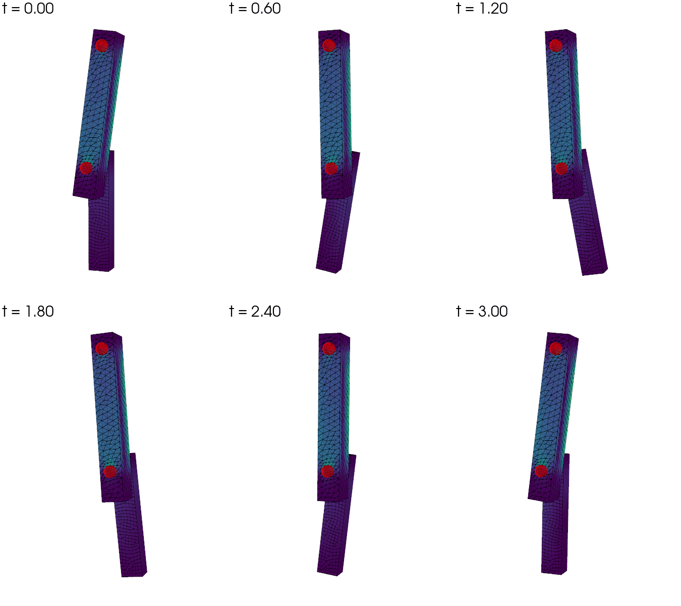
As in Anisotropic wave system with periodic boundary conditions, each process builds grids of the cells it owns, gathered once onto one process, as the meshes do not move; per frame only the nodal values and the stresses of the cells are gathered. The beams and the pins are drawn displaced by the swing \(u\) at true scale, the pins in translucent red, and the beams are coloured by the von Mises stress of the total stress, \(\sigma(u_0 + u)\): the prestress and the swing’s.
We can now perform the time stepping, writing a frame every two steps, and checking every 25 steps that the energy is conserved, as shown in the energy conservation.
history = [(0.0, *spider_turns(u_n))]
E_0 = energy(energies)
move_pins(u_n)
write_frame(0.0)
drift = 0.0
for writer in writers:
    writer.write(0.0)
for step in range(1, num_steps + 1):
    with b.localForm() as b_local:
        b_local.set(0.0)
    dolfinx_mpc.assemble_vector(L_step, mpcs, b)
    b.ghostUpdate(addv=PETSc.InsertMode.ADD_VALUES, mode=PETSc.ScatterMode.REVERSE)
    dolfinx.fem.petsc.set_bc(b, pinned_by_block)
    solver.solve(b, xh)
    xh.ghostUpdate(addv=PETSc.InsertMode.INSERT, mode=PETSc.ScatterMode.FORWARD)
    dolfinx.fem.petsc.assign(xh, u_new)
    # Every block is homogenized before any is back-substituted, as spider masters are read across blocks
    for mpc, u in zip(mpcs, u_new):
        mpc.homogenize(u)
    for mpc in mpcs:
        mpc.backsubstitution(u_new)
    # (iii): u_dot^{n+1} = 2 / dt (u^{n+1} - u^n) - u_dot^n, then u^n = u^{n+1}
    for u, u_old, u_dot in zip(u_new, u_n, u_dot_n):
        u_dot.x.array[:] = 2 / dt * (u.x.array - u_old.x.array) - u_dot.x.array
        u_old.x.array[:] = u.x.array
    history.append((step * dt, *spider_turns(u_n)))
    move_pins(u_n)
    for writer in writers:
        writer.write(step * dt)
    if step % 2 == 0:
        write_frame(step * dt)
    if step % 25 == 0:
        drift = max(drift, abs(energy(energies) / E_0 - 1))
        if comm.rank == 0:
            t, turn_1, turn_2 = history[-1]
            print(
                f"t = {t:.2f}: beam 1 at {np.rad2deg(turn_1):6.2f}°, beam 2 at {np.rad2deg(turn_2):6.2f}°,"
                f" |E / E_0 - 1| <= {drift:.1e}"
            )
for writer in writers:
    writer.close()
if comm.rank == 0:
    plotter.close()

# The PETSc objects of the step are destroyed explicitly, and those that Python's garbage
# collector has freed are cleaned up on every process together, so that no process is left
# waiting for another when PETSc finalizes
solver.destroy()
A.destroy()
b.destroy()
xh.destroy()
PETSc.garbage_cleanup(comm)
t = 0.50: beam 1 at 0.80°, beam 2 at 8.78°, |E / E_0 - 1| <= 4.7e-09
t = 1.00: beam 1 at -3.66°, beam 2 at -1.77°, |E / E_0 - 1| <= 4.7e-09
t = 1.50: beam 1 at -2.33°, beam 2 at -16.01°, |E / E_0 - 1| <= 4.7e-09
t = 2.00: beam 1 at -4.54°, beam 2 at 2.86°, |E / E_0 - 1| <= 4.7e-09
t = 2.50: beam 1 at 2.88°, beam 2 at 5.09°, |E / E_0 - 1| <= 4.7e-09
t = 3.00: beam 1 at 7.47°, beam 2 at 1.32°, |E / E_0 - 1| <= 4.7e-09
The swing, released from rest:
The energy is conserved up to the rounding of the solves, which the stiff springs next to the mass make large.
Verification invalid in single precision
The checks of the swing, here and against the rigid pendulums below, are only made in
double precision. In single precision (float32 and complex64) the swing cannot be
resolved. Its displacement is close to a large rigid turn, whose strain at a quadrature
point is the sum of terms of size \(|u| / h\) that nearly cancel. Their rounding leaves a
strain of order \(10^{-4}\), and so an elastic stress \(E \cdot 10^{-4}\) as large as the
prestress \(\sigma_0\) that drives the swing. The demo still runs, but the swing it computes
is not accurate.
if double_precision:
    assert drift < min(1e-2, 1e8 * np.finfo(default_real_type).eps)
Verification against rigid double pendulums#
Rigid beams turning by \(\varphi_1\) about the fixed pin and \(\varphi_2\) about the lower pin, for small angles, satisfy \(M_\varphi \ddot\varphi + K_\varphi \varphi = 0\). Two such models are stepped with the same midpoint rule as the beams, starting from the same turns.
The first restricts the finite element model to the two rigid turns \(R_1\) and \(R_2\), \((M_\varphi)_{ij} = M(R_i, R_j)\) and \((K_\varphi)_{ij} = \hat K(R_i, R_j)\). It differs from the beams only by their elasticity, which beam 1, the softer, shows the most.
The second is the textbook compound double pendulum,
with \(\ell = 0.8 L\) the distance between the pins, and for each beam its mass, its centre of mass, the depth of that below the beam’s pin \(x_b\) (\(x_P\) for beam 1, \(x_B\) for beam 2), and its moment of inertia about the pin, integrated over its mesh, with its bores,
Its masses are those of the first model, but not quite its stiffness, as the energy of a rigid swing shows.
Check: the energy of a rigid swing#
To see that the geometric stiffness is the pendulum’s potential, turn one beam rigidly by an angle \(\theta\) about its pin, through \(x_c\) along \(a = (0, 1, 0)\): \(u = \theta\, a \times \xi\) with \(\xi = x - x_c\). The two parts of the stored energy are then
elastic: \(\varepsilon(u) = \operatorname{sym} \nabla u = 0\), as \(\nabla u\) is the skew-symmetric matrix of \(\theta a \times\), so \(\frac12 a(u, u) = 0\);
geometric: \(\nabla u^T \nabla u = \theta^2 (I - a a^T)\), the projection onto the plane of the swing, so
\[ \frac12 a_{\sigma_0}(u, u) = \frac{\theta^2}{2} \int_{\Omega_b} \sigma_0 : (I - a a^T)~\mathrm{d}x = \frac{\theta^2}{2} \int_{\Omega_b} \left(\sigma_{0,xx} + \sigma_{0,zz}\right)~\mathrm{d}x. \]
The integral of the prestress follows from the equilibrium of the hanging beam, \(-\nabla \cdot \sigma_0 = \rho g\) in \(\Omega_b\), with the traction \(\sigma_0 n = \tau\) that the spiders exert on the bores and no traction elsewhere. Multiplying by \(\xi\) and integrating by parts gives
and taking the trace in the plane of the swing,
with \(m_b\) the mass of the beam and \(h_b\) the depth of its centre of mass below the pin, as \(g = (0, 0, -g)\) is perpendicular to \(a\). The first term gives \(\frac12 m_b g h_b \theta^2\), the exact potential of a rigid pendulum, \(m_b g h_b (1 - \cos\theta)\), to second order in \(\theta\). The bore terms add the work of the loads the beam carries:
for beam 1, the weight of beam 2 hangs from its lower bore, a distance \(\ell = 0.8 L\) below the pin, and adds \(\frac12 m_2 g \ell\, \theta^2\), as in \(K_\varphi\) of the textbook double pendulum above;
at the bore a beam hangs from, the pin’s force acts a bore radius \(r\) off the axis and adds a term of relative size \(r / h_b\). The textbook pendulum leaves this term out, so over a few swings it drifts out of phase with the beams.
So, for a swing, the stored energy \(\frac12 u \cdot \hat K u\) is the elastic energy of the beams’ deformation, \(\frac12 a(u, u)\), plus the pendulum’s potential, \(\frac12 a_{\sigma_0}(u, u)\), plus the energy of the springs, \(\frac12 s_\text{free}(w, w)\), which stays small as long as the pins hold the spiders together.
mass, centre, inertia = [], [], []
for b, (m, x_pivot) in enumerate(((beam_1, x_P), (beam_2, x_B))):
    x = ufl.SpatialCoordinate(m)
    rho = materials["rho"][b]
    mass.append(integrate(rho * ufl.dx(m)))
    centre.append(np.array([integrate(rho * x[i] * ufl.dx(m)) for i in range(3)]) / mass[-1])
    # The distance from the pin's axis, along y: its x and z components
    arm = ufl.as_vector([x[0] - x_pivot[0], x[2] - x_pivot[2]])
    inertia.append(integrate(rho * ufl.inner(arm, arm) * ufl.dx(m)))
if comm.rank == 0:
    print(f"Masses {mass[0]:.4f}, {mass[1]:.4f}; centres {centre[0].round(4)}, {centre[1].round(4)}")

ell = x_P[2] - x_B[2]
h = (x_P[2] - centre[0][2], x_B[2] - centre[1][2])
textbook = (
    np.array([[inertia[0] + mass[1] * ell**2, mass[1] * ell * h[1]], [mass[1] * ell * h[1], inertia[1]]]),
    g * np.diag([mass[0] * h[0] + mass[1] * ell, mass[1] * h[1]]),
)

modes = [[fem.Function(mpc.function_space, dtype=default_scalar_type) for mpc in mpcs] for _ in range(3)]
# Beam 2 turned by phi_2 in all, so that both models use the absolute turns
rigid_turns(1.0, -1.0, modes[0])
rigid_turns(0.0, 1.0, modes[1])
zero = [fem.Function(mpc.function_space, dtype=default_scalar_type) for mpc in mpcs]


def quadratic(i: int, j: int, kinetic: bool) -> float:
    """M(R_i, R_j) if `kinetic`, else K(R_i, R_j), by polarization of the energy."""
    for f, f_i, f_j in zip(modes[2], modes[i], modes[j]):
        f.x.array[:] = f_i.x.array + f_j.x.array

    def twice_energy(u):
        return 2 * energy(energy_forms(zero, u) if kinetic else energy_forms(u, zero))

    return 0.5 * (twice_energy(modes[2]) - twice_energy(modes[i]) - twice_energy(modes[j]))


ritz = tuple(np.array([[quadratic(i, j, kinetic) for j in range(2)] for i in range(2)]) for kinetic in (True, False))


def swing(M_phi: np.ndarray, K_phi: np.ndarray) -> np.ndarray:
    """The turns of a rigid double pendulum, stepped as the beams were."""
    step_matrix = np.linalg.inv(4 / dt**2 * M_phi + K_phi)
    phi, phi_dot, phi_new = np.array([theta_1, theta_1 + theta_2]), np.zeros(2), np.zeros(2)
    # The initial turns, and those after each step
    turns = np.zeros((num_steps + 1, 2))
    turns[0] = phi
    for step in range(1, num_steps + 1):
        phi_new[:] = step_matrix @ (4 / dt**2 * M_phi @ phi + 4 / dt * M_phi @ phi_dot - K_phi @ phi)
        phi_dot[:] = 2 / dt * (phi_new - phi) - phi_dot
        phi[:] = phi_new
        turns[step] = phi
    return turns


turns = np.array(history)[:, 1:]
mismatch = {
    name: np.abs(turns - swing(*model)).max() / np.abs(turns).max()
    for name, model in (("ritz", ritz), ("textbook", textbook))
}
mass_difference = np.abs(ritz[0] - textbook[0]).max() / np.abs(textbook[0]).max()
stiffness_difference = np.diag(ritz[1]) / np.diag(textbook[1]) - 1
if comm.rank == 0:
    print(f"Masses, relative to the textbook pendulum's: {mass_difference:.1e}")
    print(f"Stiffness, relative to the textbook pendulum's: {stiffness_difference.round(3)}")
    print(
        f"Largest difference of the turns to the rigid pendulums: {mismatch['ritz']:.1%} (finite elements),"
        f" {mismatch['textbook']:.1%} (textbook)"
    )
Masses 0.2479, 0.1470; centres [ 0. 0.2 -0.9065], [-0. 0.575 -2.2767]
Masses, relative to the textbook pendulum's: 8.3e-14
Stiffness, relative to the textbook pendulum's: [-0.061 -0.058]
Largest difference of the turns to the rigid pendulums: 2.1% (finite elements), 17.7% (textbook)
The masses agree to rounding, the stiffnesses to the order of \(r / h\), and the beams follow the rigid pendulum of the finite element model to a few percent. As noted above, the last two are only checked in double precision.
assert mass_difference < 1e4 * np.finfo(default_real_type).eps
if double_precision:
    assert np.all(np.abs(stiffness_difference) < radius / min(h))
    assert mismatch["ritz"] < 0.1
Finally, the static problem’s PETSc objects are released and cleaned up in the same way.