Advanced finite elements#
There is a wide range of finite elements that are supported by ufl and basix. See for instance: Supported elements in basix/ufl.
Domain mapping#
The general idea of the finite element method is to sub-divide \(\Omega\) into smaller (polygonal) elements \(K_j\) such that
The triangulation covers \(\Omega\): \(\cup_{j=1}^{M}K_j=\bar{\Omega}\)
No overlapping polyons: \(\mathrm{int} K_i \cap \mathrm{int} K_j=\emptyset\) for \(i\neq j\).
No vertex lies in the interior of a facet or edge of another element
We will call our polygonal domain \(\mathcal{K}=\{K_j\}_{j=1}^{M}\). Next, we define a reference element \(K_{ref}\), which is a simple polygon that we can map to any element \(K_j\), using the mapping \(F_j:K_{ref}\mapsto K_j\).
We define the Jacobian of this mapping as \(\mathbf{J_j}\).
Example: Straight edged triangle#
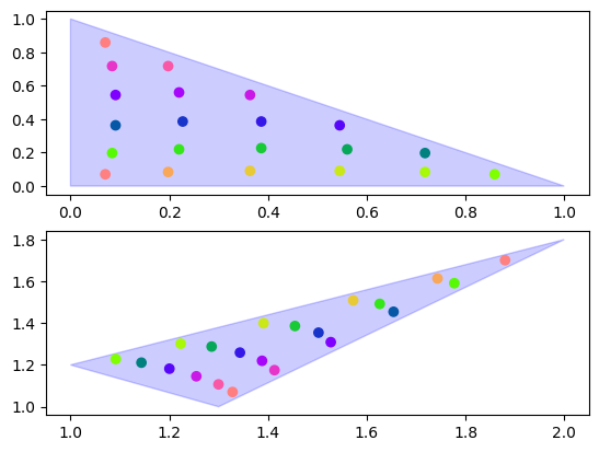
As we saw in the section on finite elements, we can use basix to get a sample of points within the reference element.
import numpy as np

import basix.ufl

reference_points = basix.create_lattice(
    basix.CellType.triangle, 8, basix.LatticeType.gll, exterior=False, method=basix.LatticeSimplexMethod.warp
)
Next, we realize that we can use the first order Lagrange space, to represent the mapping from the reference element to any physical element: Given three points, \(\mathbf{p}_0=(x_0, y_0)^T, \mathbf{p}_1=(x_1,y_1)^T, \mathbf{p}_2=(x_2,y_2)^T\), we can represent any point \(x\) as the linear combination of the three basis functions on the reference element \(X\).
In the next snippet we will create a function to compute x given the three points and a set of reference coordinates
def compute_physical_point(p0, p1, p2, X):
    """
    Map coordinates `X` in reference element to triangle defined by `p0`, `p1` and `p2`
    """
    el = basix.ufl.element("Lagrange", "triangle", 1)
    basis_values = el.tabulate(0, X)
    x = basis_values[0] @ np.vstack([p0, p1, p2])
    return x
We can now experiment with this code
Reference points: [[0.07049245 0.07049245]
 [0.19773226 0.08429537]
 [0.3635668  0.09126483]
 [0.54516837 0.09126483]
 [0.71797237 0.08429537]
 [0.8590151  0.07049245]
 [0.08429537 0.19773226]
 [0.21983534 0.21983534]
 [0.38637247 0.22725505]
 [0.56032931 0.21983534]
 [0.71797237 0.19773226]
 [0.09126483 0.3635668 ]
 [0.22725505 0.38637247]
 [0.38637247 0.38637247]
 [0.54516837 0.3635668 ]
 [0.09126483 0.54516837]
 [0.21983534 0.56032931]
 [0.3635668  0.54516837]
 [0.08429537 0.71797237]
 [0.19773226 0.71797237]
 [0.07049245 0.8590151 ]]
Physical points: [[1.88016284 1.70131057]
 [1.74326098 1.61392435]
 [1.57254782 1.50884806]
 [1.39094625 1.39988711]
 [1.22302087 1.30178028]
 [1.09164018 1.22819698]
 [1.77729205 1.59123697]
 [1.62627992 1.49223052]
 [1.45454899 1.38637247]
 [1.28578595 1.28793414]
 [1.14361504 1.21103077]
 [1.65423841 1.45438766]
 [1.50228422 1.35454899]
 [1.34316679 1.25907854]
 [1.20033487 1.18204554]
 [1.52711731 1.3091064 ]
 [1.38793414 1.21983534]
 [1.25481534 1.14572522]
 [1.41312397 1.17504488]
 [1.29968708 1.10698275]
 [1.32819698 1.07049245]]
We use matplotlib to visualize the reference points and the physical points
Exercises:#
Can we use a similar kind of mapping on a quadrilateral/tetrahedral/hexahedral element?
Yes, as long as we can describe the shape with a Lagrange finite element, we can define a mapping from a reference to a physical element.
What happens if we change the degree of the basis functions?
We require more nodes to describe our polygon. For instance, if we use a second order Lagrange element on a triangle, we would require 3 additional nodes to describe the midpoint of each edge.
How can we compute the Jacobian of the mapping?
As we now have an expression \(F=x(X)\), we can compute the Jacobian by taking the derivative of \(F\) with respect to \(x\), i.e. \(J = \frac{\partial F}{\partial X}=\sum_{i=0}^3 \mathbf{p}_i (\nabla \phi_i(X))^T\).
Mapping of basis functions from the reference element#
As we have already seen, we can describe any cell in our subdivided domain with a mapping from the reference element. However, as we want to integrate over each element individually, we need to map the basis functions to and from the reference element. We call this map: \((\mathcal{F}_j\phi)(x)\).
For scalar valued basis functions, such as the Lagrange basis function, this operation is simple
Vector-valued finite elements#
The basis functions we have considered so far have been scalar-valued, i.e. for each DOF \(u_i\) we have a scalar valued basis function \(\phi_i\).
In this section we will consider vector-valued basis functions
Instead of defining the dual basis \(l_i\) as point evaluations, these dual-basis functions are often defined as integrals over a sub-entity of the reference cell, i.e. an edge, facet or the cell itself.
We will considered the finite element called Nédélec (first kind). For simplicity we will consider the first order element on a triangle, where:
where \(t_i\) is the tangent to the edge \(e_i\).
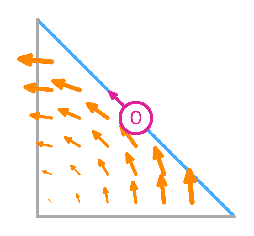
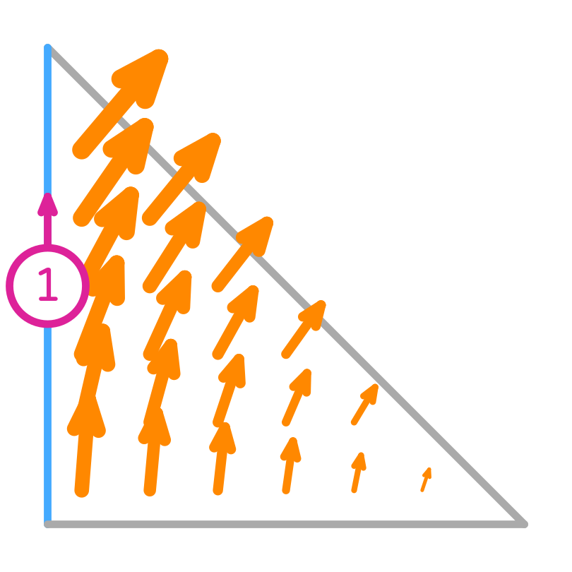
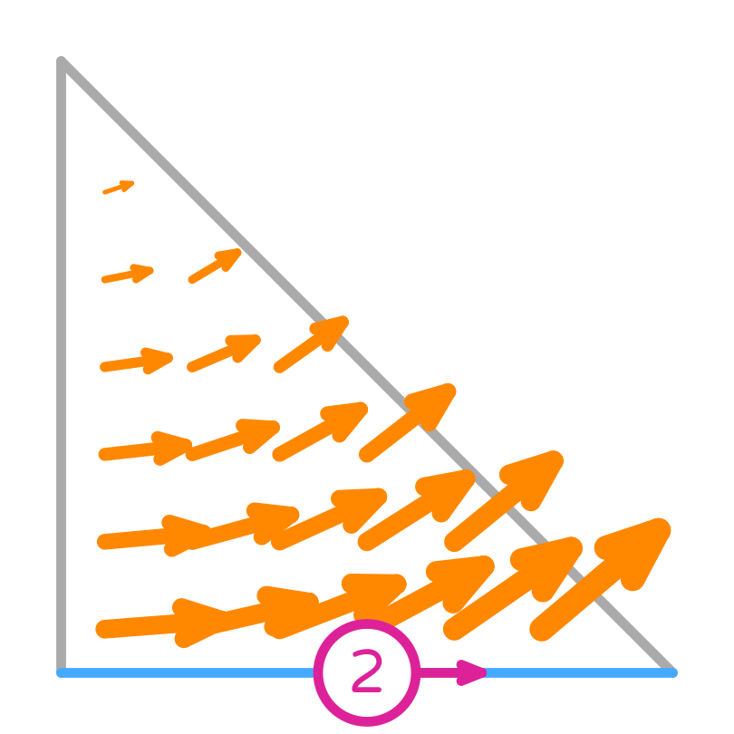
Nédélec (first kind) basis functions
What properties do the basis functions above have?
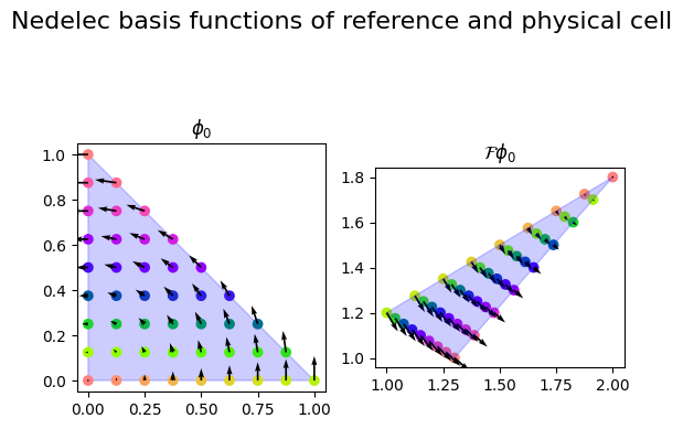
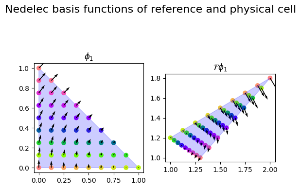
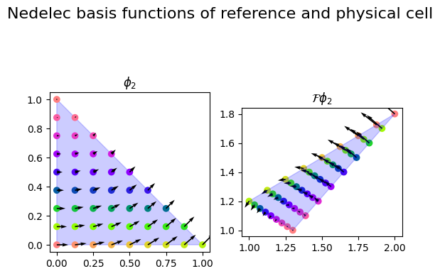
Their tangential component is only non-zero on the edge they are associated with, but the normal component can be non-zero there too. This implies that they are normal to the other edges.
To preserve the properties of the basis functions from the reference element to the physical element, we use the covariant Piola map:
The noteable feature of this map is that it preserves the tangential component of the basis function. We start by computing the Jacobian of the mapping from the reference element to the physical element.
Tabulating vector valued basis functions with basix
When the basis function is vector-valued, basix returns the basis functions with the shape
(num_derivatives, num_points, vector_dimension, num_basis_functions).
Exercise: Compute the Jacobian of the mapping from the reference element to the physical element at a single point in the reference element#
Expand to reveal the solution
If we use a straight edged triangle, is the Jacobian spatially dependent?
No, the Jacobian is constant over the entire element, as the mapping is affine. If we instead considered a general quadrilateral or hexahedral element, the Jacobian would be spatially dependent. It is only constant in the setting where the quadrilateral is a parallelogram or the hexahedron is a parallelepiped.
Exercise: Compute \(J^{-T}\)#
Expand to reveal the solution
Exercise: Tabulate the basis functions of a first order Nedelec element on the reference element#
Expand to reveal the solution
We can visualize the basis functions side by side
Exercise#
What property does the covariant Piola mapping preserve?
We observe that the covariant Piola map maps normals to normals, since a 0 tangential component is mapped to a 0 tangent.
Why are these elements useful?
The Maxwell’s equations can be written as
where \(\mathbf{E}\) is the electric field, \(\mathbf{B}\) is the magnetic field, \(\mathbf{J}\) is the current density, \(\rho\) is the electric charge density, \(\epsilon_0\) the vacuum permittivity, and \(\mu_0\) the vacuum permeability.
The normal component of the \(\mathbf{B}\)-field is always continuous, while the tangential component is discontinuous across a material interface. Similarly, the \(\mathbf{H}\)-field is related to \(\mathbf{B}\) by \(\mathbf{H}=\frac{1}{\mu}(\mathbf{B}-\mathbf{M})\), where \(\mathbf{M}\) is the magnetization. This field has continuous tangential components and discontinuous normal components, which is suitable for the Nédélec (first kind) element.