Generating code for assembling tensors

All the code in the previous section is Python code that is a symbolic representation the variational form of a projection.

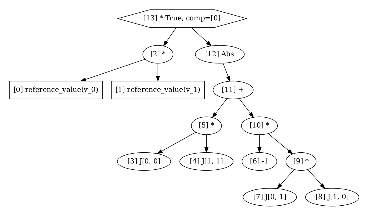
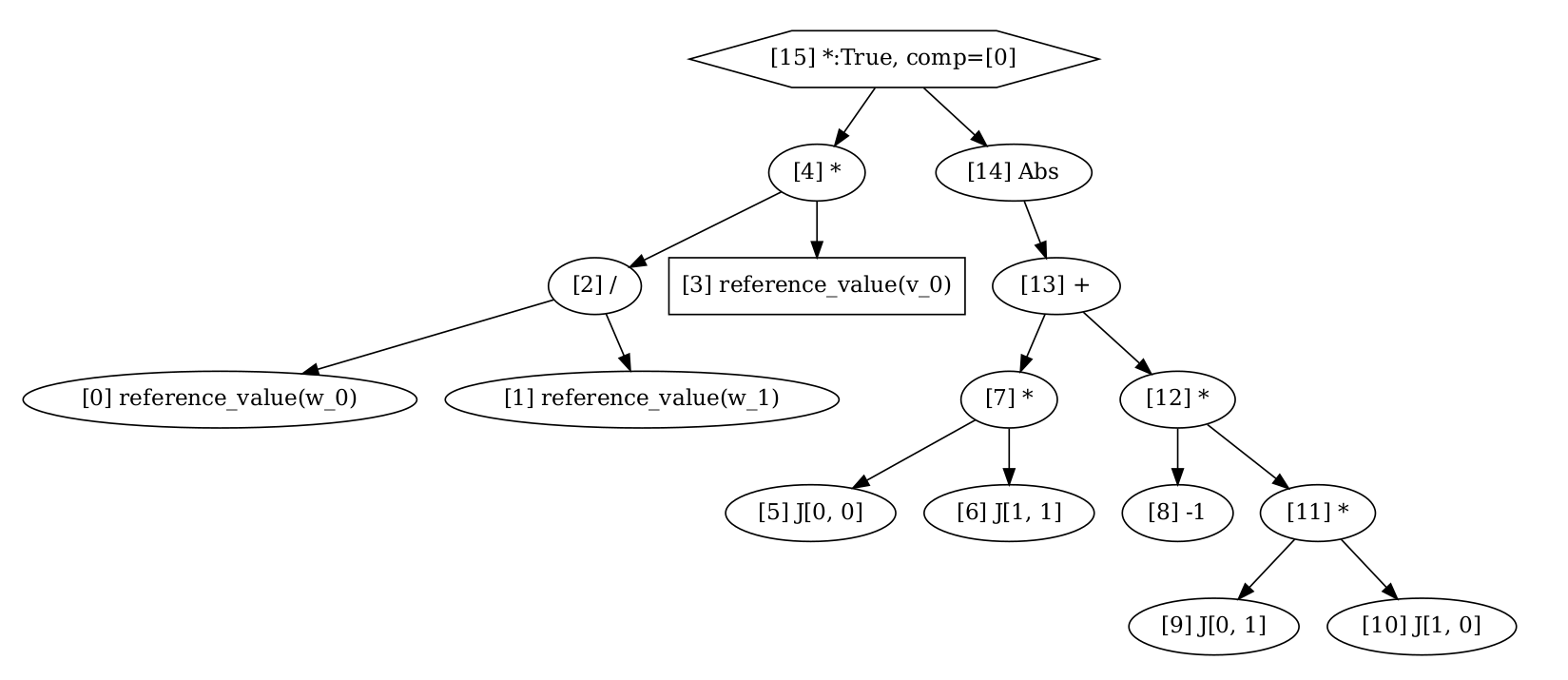
Creating code for each and every variational formulation is a tedious task, and it is error-prone. Therefore, in FEniCS, we exploit the symbolic representation of a variational form to generate code for assembling local element tensors. One can interpret the variational form written in UFL as a directed acyclic graph (DAG) of operations, where each operation can be implemented in C.

The FEniCSx Form Compiler (FFCx)

We use FFCx to generate the code used for finite element assembly.

The previous section of the tutorial can be found in the file example.py. We can use the FFCx main-module to generate C code for all the objects in this file:

import os
from pathlib import Path

import ffcx.main

infile = Path.cwd() / "example.py"

_ = os.system(f"cat {infile}")

import basix.ufl
import ufl

cell = "triangle"
c_el = basix.ufl.element("Lagrange", cell, 1, shape=(2,))
domain = ufl.Mesh(c_el)

el = basix.ufl.element("Lagrange", cell, 2)
V = ufl.FunctionSpace(domain, el)
u = ufl.TrialFunction(V)
v = ufl.TestFunction(V)

a = ufl.inner(u, v) * ufl.dx

forms = [a]

ffcx.main.main(["-o", str(infile.parent), "--visualise", str(infile)])

What happens when we run the command above? The first thing that happens is that each line of code in the file is executed by the Python interpreter. Then, all variational formulations that have been given the name a, L or J is being extracted.

Note

If you only want to extract a specific form, or a form that is not named as above, create a list called forms and add the form to this list.

For each of this forms, FFCx uses UFL to convert the initial expression into a low level representation with the DAG, and then generates C code for the assembly of the local element tensors. This computes the computational graph of the bi-linear and linear form

Bilinear graph

Linear graph

The generated code can be found in the file name_of_file.h and name_of_file.c in the current working directory.

_ = os.system(f"ls {infile.with_suffix('.*')}")

/__w/FEniCS-workshop/FEniCS-workshop/src/example.c
/__w/FEniCS-workshop/FEniCS-workshop/src/example.h
/__w/FEniCS-workshop/FEniCS-workshop/src/example.py

We can look at the assembly code for the local matrix. We start by inspecting the signature of the tabulate_tensor function that computes the local element matrix

_ = os.system(f"head -102 {infile.with_suffix('.c')} | tail +28")

void tabulate_tensor_integral_9acfb88b3b905b01b19619a14c68c3b8c39f1c46(double* restrict A,
                                    const double* restrict w,
                                    const double* restrict c,
                                    const double* restrict coordinate_dofs,
                                    const int* restrict entity_local_index,
                                    const uint8_t* restrict quadrature_permutation)
{
// Quadrature rules
static const double weights_39d[6] = {0.054975871827661, 0.054975871827661, 0.054975871827661, 0.1116907948390055, 0.1116907948390055, 0.1116907948390055};
// Precomputed values of basis functions and precomputations
// FE* dimensions: [permutation][entities][points][dofs]
static const double FE0_C0_Q39d[1][1][6][6] = {{{{-0.07480380774819603, 0.5176323419876736, -0.07480380774819671, 0.2992152309927871, 0.03354481152314834, 0.2992152309927839},
  {-0.07480380774819613, -0.0748038077481966, 0.5176323419876735, 0.2992152309927871, 0.2992152309927838, 0.03354481152314828},
  {0.5176323419876713, -0.0748038077481967, -0.07480380774819674, 0.03354481152314866, 0.2992152309927869, 0.2992152309927868},
  {-0.04820837781551195, -0.08473049309397784, -0.04820837781551192, 0.1928335112620479, 0.7954802262009061, 0.1928335112620478},
  {-0.04820837781551193, -0.048208377815512, -0.08473049309397786, 0.1928335112620479, 0.192833511262048, 0.7954802262009062},
  {-0.08473049309397794, -0.04820837781551188, -0.04820837781551195, 0.7954802262009061, 0.1928335112620479, 0.1928335112620479}}}};
static const double FE2_C0_D10_Q39d[1][1][1][3] = {{{{-1.0, 1.0, 0.0}}}};
static const double FE2_C1_D01_Q39d[1][1][1][3] = {{{{-1.0, 0.0, 1.0}}}};
// ------------------------ 
// Section: Jacobian
// Inputs: coordinate_dofs, FE2_C0_D10_Q39d, FE2_C1_D01_Q39d
// Outputs: J_c1, J_c2, J_c3, J_c0
double J_c0 = 0.0;
double J_c3 = 0.0;
double J_c1 = 0.0;
double J_c2 = 0.0;
{
  for (int ic = 0; ic < 3; ++ic)
  {
    J_c0 += coordinate_dofs[(ic) * 3] * FE2_C0_D10_Q39d[0][0][0][ic];
    J_c3 += coordinate_dofs[(ic) * 3 + 1] * FE2_C1_D01_Q39d[0][0][0][ic];
    J_c1 += coordinate_dofs[(ic) * 3] * FE2_C1_D01_Q39d[0][0][0][ic];
    J_c2 += coordinate_dofs[(ic) * 3 + 1] * FE2_C0_D10_Q39d[0][0][0][ic];
  }
}
// ------------------------ 
double sp_39d_0 = J_c0 * J_c3;
double sp_39d_1 = J_c1 * J_c2;
double sp_39d_2 = -sp_39d_1;
double sp_39d_3 = sp_39d_0 + sp_39d_2;
double sp_39d_4 = fabs(sp_39d_3);
for (int iq = 0; iq < 6; ++iq)
{
  // ------------------------ 
  // Section: Intermediates
  // Inputs: 
  // Outputs: fw0
  double fw0 = 0;
  {
    fw0 = sp_39d_4 * weights_39d[iq];
  }
  // ------------------------ 
  // ------------------------ 
  // Section: Tensor Computation
  // Inputs: fw0, FE0_C0_Q39d
  // Outputs: A
  {
    double temp_0[6] = {0};
    for (int j = 0; j < 6; ++j)
    {
      temp_0[j] = fw0 * FE0_C0_Q39d[0][0][iq][j];
    }
    for (int j = 0; j < 6; ++j)
    {
      for (int i = 0; i < 6; ++i)
      {
        A[6 * (i) + (j)] += FE0_C0_Q39d[0][0][iq][i] * temp_0[j];
      }
    }
  }
  // ------------------------ 
}

}

Optional Exercise

Study the computational graph for the bi-linear form, and the kernel for the assembly of this form below. Do you understand each step?