Mesh generation

We have now covered the most basic aspects of setting up a problem in DOLFINx. We can now look into how to solve specific problems. Let us start with generating the computational domain.

Create a mesh with numpy arrays

In DOLFINx, the mesh creation requires 4 inputs:

• MPI communicator: This is used to decide how the partitioning is performed. It is usually MPI.COMM_WORLD or MPI.COMM_SELF.

• Nodes: A set of coordinates in 1, 2 or 3D, that represents all the points in the mesh

• Connectivity: A nested list, where each row corresponds to the node indices of a single cell

• Coordinate element: A finite element used for pushing coordinates from the reference element to the physical element and its inverse.

We start by importing the necessary modules for this section

from mpi4py import MPI

import matplotlib.pyplot as plt
import numpy as np
import pyvista

import basix.ufl
import dolfinx
import ufl

As an example, let us consider a simple two element mesh, of two straight edged triangles. We start by creating the four nodes that the grid will consist of

nodes = np.array([[1.0, 0.0], [2.0, 0.0], [3.0, 2.0], [1, 3]], dtype=np.float64)

Next, we define each cell by the index of the row each point has in the nodes-array

connectivity = np.array([[0, 1, 2], [0, 2, 3]], dtype=np.int64)

As we have seen in the previous section we use a finite element to describe the mapping from the reference triangles to the physical triangles described above.

c_el = ufl.Mesh(basix.ufl.element("Lagrange", "triangle", 1, shape=(nodes.shape[1],)))

Finally we create a mesh object by calling dolfinx.mesh.create_mesh with the aforementioned inputs

domain = dolfinx.mesh.create_mesh(MPI.COMM_SELF, connectivity, nodes, c_el)

Visualizing the mesh

The mesh can be visualized with Paraview or Pyvista.

Press the drop-down button to inspect the code for visualizing the mesh

Show code cell source Hide code cell source

def plot_mesh(mesh: dolfinx.mesh.Mesh, values=None):
    """
    Given a DOLFINx mesh, create a `pyvista.UnstructuredGrid`,
    and plot it and the mesh nodes.

    Args:
        mesh: The mesh we want to visualize
        values: List of values indicating a marker for each cell in the mesh

    Note:
        If `values` are given as input, they are assumed to be a marker
        for each cell in the domain.
    """
    # We create a pyvista plotter instance
    plotter = pyvista.Plotter()

    # Since the meshes might be created with higher order elements,
    # we start by creating a linearized mesh for nicely inspecting the triangulation.
    V_linear = dolfinx.fem.functionspace(mesh, ("Lagrange", 1))
    linear_grid = pyvista.UnstructuredGrid(*dolfinx.plot.vtk_mesh(V_linear))

    # If the mesh is higher order, we plot the nodes on the exterior boundaries,
    # as well as the mesh itself (with filled in cell markers)
    if mesh.geometry.cmap.degree > 1:
        ugrid = pyvista.UnstructuredGrid(*dolfinx.plot.vtk_mesh(mesh))
        if values is not None:
            ugrid.cell_data["Marker"] = values
        plotter.add_mesh(ugrid, style="points", color="b", point_size=10)
        ugrid = ugrid.tessellate()
        plotter.add_mesh(ugrid, show_edges=False)
        plotter.add_mesh(linear_grid, style="wireframe", color="black")
    else:
        # If the mesh is linear we add in the cell markers
        if values is not None:
            linear_grid.cell_data["Marker"] = values
        plotter.add_mesh(linear_grid, show_edges=True)

    # We plot the coordinate axis and align it with the xy-plane
    plotter.show_axes()
    plotter.view_xy()
    plotter.show()

The mesh we created above is visualized as

Show code cell source Hide code cell source

import sys, os

if sys.platform == "linux" and (os.getenv("CI") or pyvista.OFF_SCREEN):
    pyvista.start_xvfb(0.05)
plot_mesh(domain)

Higher order meshes

As we use a finite element to describe the mapping from the reference element to the physical element, we can use higher order elements to describe the reference element, giving us the possibility to create curved meshes. In the following example,w e will create a single cell mesh (triangle) using a second order Lagrange element.

This finite element has a total of 6 degrees of freedom, and we will use the standard dual basis:

\[\begin{split} \begin{align} l_0:& v \mapsto v(0, 0) \\ l_1:& v \mapsto v(1, 0) \\ l_2:& v \mapsto v(0, 1) \\ l_3:& v \mapsto v(0.5, 0.5) \\ l_4:& v \mapsto v(0, 0.5) \\ l_6:& v \mapsto v(0.5, 0) \end{align} \end{split}\]

We will create a set of six nodes, where we follow the ordering of the dual basis functions

nodes = np.array(
    [[1.0, 0.0], [2.0, 0.0], [3.0, 2.0], [2.5, 1], [1.5, 1.5], [1.5, -0.2]],
    dtype=np.float64,
)
connectivity = np.array([[0, 1, 2, 3, 4, 5]], dtype=np.int64)

The input node ordering

We follow the node ordering of DefElement for the input order of the nodes. If you are reading in data from another format (VTK or GMSH), you can use the functions dolfinx.cpp.io.perm_vtk or dolfinx.cpp.perm_gmsh to get the map from the ordering of the nodes from the aforementioned formats to DOLFINx. You would apply this as

connectivity_dolfinx = connectivity_vtk[perm_vtk(...)]
connectivity_dolfinx = connectivity_gmsh[perm_gmsh(...)]

To convert from the DOLFINx ordering to either VTK or GMSH, you would use the inverse permutation with np.argsort(perm_vtk(...)).

With this in mind, we can create the DOLFINx mesh

c_el = ufl.Mesh(basix.ufl.element("Lagrange", "triangle", 2, shape=(nodes.shape[1],)))
domain = dolfinx.mesh.create_mesh(MPI.COMM_SELF, connectivity, nodes, c_el)

Questions/Exercises

1. Where are the point evaluations \(l_3, l_4, l_5\) located in the reference triangle?

2. Which entities do we associate each functional with?

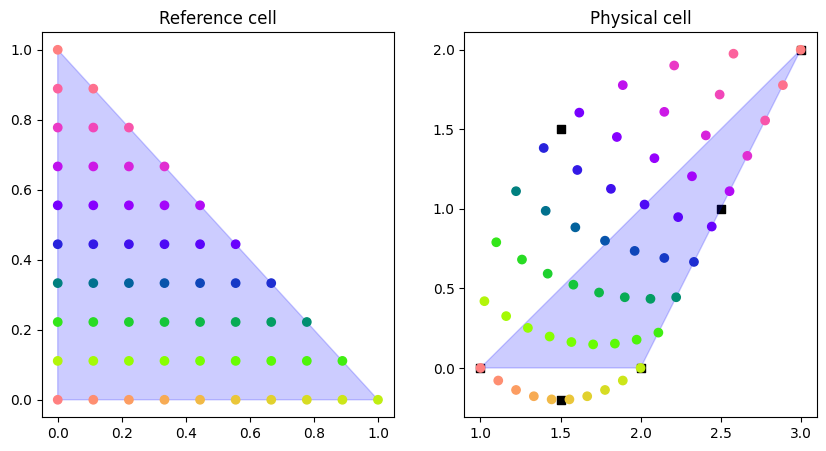
3. Can you make a visualization script for the push forward from the reference element to the a physical element, as done in Example: Straight edged triangle?

Press the following dropdown to reveal the solution to exercise 3.

Show code cell source Hide code cell source

def compute_physical_point(points, X, degree: int = 2):
    """
    Map coordinates `X` in reference element to triangle defined by `p0`, `p1` and `p2`
    """
    el = basix.ufl.element("Lagrange", "triangle", degree)
    basis_values = el.tabulate(0, X)
    assert points.shape[0] == basis_values.shape[2], "Nodes not matching finite element basis functions"
    return basis_values[0] @ points

Expand the next dropdown to see how to plot the nodes on the reference and physical cell

Show code cell source Hide code cell source

# Create equispaced points on the reference triangle
theta = 2 * np.pi
reference_points = basix.create_lattice(basix.CellType.triangle, 9, basix.LatticeType.equispaced, exterior=True)
# Compute push forward
x = compute_physical_point(nodes, reference_points, degree=2)

# Create a unique colors for each node
phi = np.linspace(0, theta, reference_points.shape[0])
rgb_cycle = (np.stack((np.cos(phi), np.cos(phi - theta / 4), np.cos(phi + theta / 4))).T + 1) * 0.5

# Create a 1x2 plot
fig, (ax_ref, ax) = plt.subplots(1, 2, figsize=(10, 5))
ax_ref.set_title("Reference cell")

# Plot reference points
reference_vertices = basix.cell.geometry(basix.CellType.triangle)
ref_triangle = plt.Polygon(reference_vertices, color="blue", alpha=0.2)
ax_ref.add_patch(ref_triangle)
ax_ref.scatter(reference_points[:, 0], reference_points[:, 1], c=rgb_cycle)

# Plot physical points
triangle = plt.Polygon(nodes[[0, 1, 2]], color="blue", alpha=0.2)

# Plot all nodes
ax.set_title("Physical cell")
ax.scatter(nodes[:, 0], nodes[:, 1], color="black", marker="s")
ax.add_patch(triangle)
ax.scatter(x[:, 0], x[:, 1], c=rgb_cycle)

<matplotlib.collections.PathCollection at 0x7f0f4f1aa630>

We use the convenience function from above to visualize the mesh with Pyvista

plot_mesh(domain)