Approximation with continuous and discontinuous finite elements

Approximation with continuous and discontinuous finite elements#

We introduced the notion of a projection in The variational form of a projection where we want to find the best approximation of an expression in a finite element space.

The goal of this section is to approximate

\[\begin{split} h(x) = \begin{cases} \cos(\pi x) \quad\text{if } x<\alpha\\ -\sin(x) \quad\text{otherwise} \end{cases} \end{split}\]

where \(\alpha\) is a pre-defined constant. We will use ufl.conditional as explained in the the previous section.

from mpi4py import MPI
from petsc4py import PETSc
import dolfinx.fem.petsc
import ufl

def h(alpha, mesh: dolfinx.mesh.Mesh):
    x = ufl.SpatialCoordinate(mesh)
    return ufl.conditional(ufl.lt(x[0], alpha), ufl.cos(ufl.pi * x[0]), -ufl.sin(x[0]))

Reusable projector#

Imagine we want to solve a sequence of such post-processing steps for functions \(f\) and \(g\). If the mesh is not changing between each projection, the left hand side is constant. Thus, it would make sense to assemble the matrix once. Following this, we create a general projector class (class Projector)

Show code cell source Hide code cell source

from typing import Optional

import numpy as np
import pyvista

class Projector:
    """
    Projector for a given function.
    Solves Ax=b, where

    .. highlight:: python
    .. code-block:: python

        u, v = ufl.TrialFunction(Space), ufl.TestFunction(space)
        dx = ufl.Measure("dx", metadata=metadata)
        A = inner(u, v) * dx
        b = inner(function, v) * dx(metadata=metadata)

    Args:
        function: UFL expression of function to project
        space: Space to project function into
        petsc_options: Options to pass to PETSc
        jit_options: Options to pass to just in time compiler
        form_compiler_options: Options to pass to the form compiler
        metadata: Data to pass to the integration measure
    """

    _A: PETSc.Mat  # The mass matrix
    _b: PETSc.Vec  # The rhs vector
    _lhs: dolfinx.fem.Form  # The compiled form for the mass matrix
    _ksp: PETSc.KSP  # The PETSc solver
    _x: dolfinx.fem.Function  # The solution vector
    _dx: ufl.Measure  # Integration measure

    def __init__(
        self,
        space: dolfinx.fem.FunctionSpace,
        petsc_options: Optional[dict] = None,
        jit_options: Optional[dict] = None,
        form_compiler_options: Optional[dict] = None,
        metadata: Optional[dict] = None,
    ):
        petsc_options = {} if petsc_options is None else petsc_options
        jit_options = {} if jit_options is None else jit_options
        form_compiler_options = {} if form_compiler_options is None else form_compiler_options

        # Assemble projection matrix once
        u = ufl.TrialFunction(space)
        v = ufl.TestFunction(space)
        self._dx = ufl.Measure("dx", domain=space.mesh, metadata=metadata)
        a = ufl.inner(u, v) * self._dx(metadata=metadata)
        self._lhs = dolfinx.fem.form(a, jit_options=jit_options, form_compiler_options=form_compiler_options)
        self._A = dolfinx.fem.petsc.assemble_matrix(self._lhs)
        self._A.assemble()

        # Create vectors to store right hand side and the solution
        self._x = dolfinx.fem.Function(space)
        self._b = dolfinx.fem.Function(space)

        # Create Krylov Subspace solver
        self._ksp = PETSc.KSP().create(space.mesh.comm)
        self._ksp.setOperators(self._A)

        # Set PETSc options
        prefix = f"projector_{id(self)}"
        opts = PETSc.Options()
        opts.prefixPush(prefix)
        for k, v in petsc_options.items():
            opts[k] = v
        opts.prefixPop()
        self._ksp.setFromOptions()
        for opt in opts.getAll().keys():
            del opts[opt]

        # Set matrix and vector PETSc options
        self._A.setOptionsPrefix(prefix)
        self._A.setFromOptions()
        self._b.x.petsc_vec.setOptionsPrefix(prefix)
        self._b.x.petsc_vec.setFromOptions()

    def reassemble_lhs(self):
        dolfinx.fem.petsc.assemble_matrix(self._A, self._lhs)
        self._A.assemble()

    def assemble_rhs(self, h: ufl.core.expr.Expr):
        """
        Assemble the right hand side of the problem
        """
        v = ufl.TestFunction(self._b.function_space)
        rhs = ufl.inner(h, v) * self._dx
        rhs_compiled = dolfinx.fem.form(rhs)
        self._b.x.array[:] = 0.0
        dolfinx.fem.petsc.assemble_vector(self._b.x.petsc_vec, rhs_compiled)
        self._b.x.petsc_vec.ghostUpdate(addv=PETSc.InsertMode.ADD_VALUES, mode=PETSc.ScatterMode.REVERSE)
        self._b.x.petsc_vec.ghostUpdate(addv=PETSc.InsertMode.INSERT_VALUES, mode=PETSc.ScatterMode.FORWARD)

    def project(self, h: ufl.core.expr.Expr) -> dolfinx.fem.Function:
        """
        Compute projection using a PETSc KSP solver

        Args:
            assemble_rhs: Re-assemble RHS and re-apply boundary conditions if true
        """
        self.assemble_rhs(h)
        self._ksp.solve(self._b.x.petsc_vec, self._x.x.petsc_vec)
        return self._x

    def __del__(self):
        self._A.destroy()
        self._ksp.destroy()

With this class, we can send in any expression written in UFL to the projector, and then generate code for the right hand side assembly, and then solve the linear system. If we use LU factorization, most of the cost will be in the first projection, when the matrix is factorized. This is then cached, so that the solution algorithm is reduced to solving to linear problems; one upper diagonal matrix and one lower diagonal matrix.

Non-aligning discontinuity#

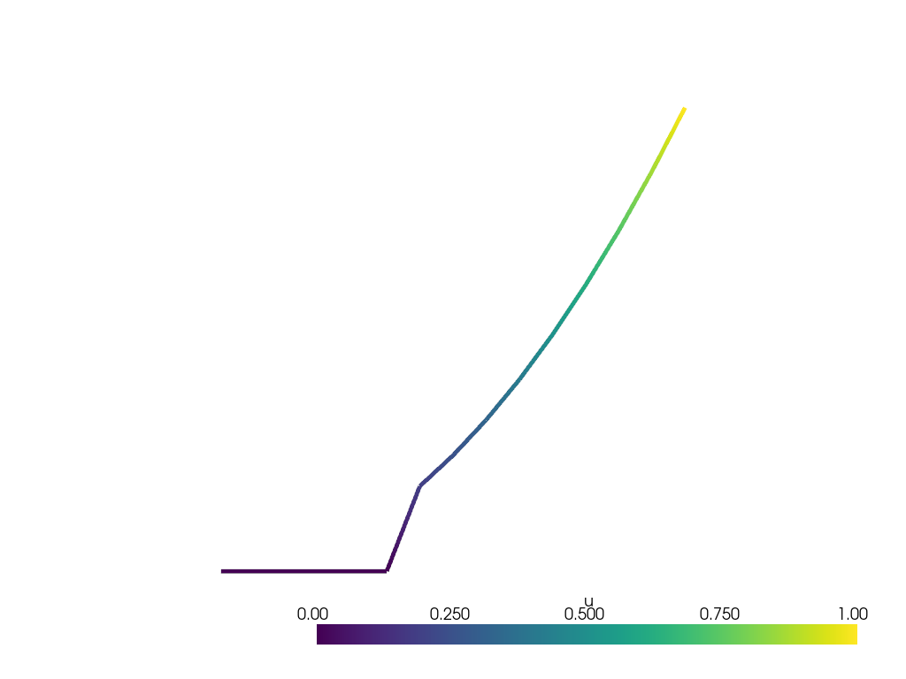
We will start considering the case where \(\alpha\) is not aligned with the mesh. We choose \(\alpha = \frac{\pi}{10}\) and get the following \(h\):

\[\begin{split} h(x) = \begin{cases} \cos(\pi x) \quad\text{if } x<\frac{\pi}{10}\\ -\sin(x) \quad\text{otherwise} \end{cases} \end{split}\]

The partial-function

For the next cases, we would like to fix alpha in our function h, but we want to keep the mesh as a variable. We can use the partial function from the functools module to fix the first argument of a function. It creates a new object that behaves as a function where mesh is the only input parameter. i.e.

from functools import partial
def f(x, y, z):
  print(f"{x=}, {y=}, {z=}")
h = partial(f, 3, 4)
h(7) # prints x=3, y=4, z=7

from functools import partial
h_nonaligned = partial(h, np.pi / 10)

Let us now try to use the re-usable projector to approximate this function with a continuous Lagrange space of order 1

Nx = 20
mesh = dolfinx.mesh.create_unit_interval(MPI.COMM_WORLD, Nx)
V = dolfinx.fem.functionspace(mesh, ("Lagrange", 1))

petsc_options={"ksp_type": "preonly", "pc_type": "lu"}
V_projector = Projector(V, petsc_options=petsc_options)
uh = V_projector.project(h_nonaligned(V.mesh))

We can now repeat the study for a discontinuous Lagrange space of order 1

W = dolfinx.fem.functionspace(mesh, ("DG", 1))
W_projector = Projector(W, petsc_options=petsc_options)
wh = W_projector.project(h_nonaligned(W.mesh))

We compare the two solutions side by side

../_images/4fccb3b1e63e8b1b165aaeddf581146d39bad23ff1db85f71c96701bdc33cd6a.png

We observe that both solutions overshoot and undershoot around the discontinuity Let us refine the mesh several times to see if the solution converges

../_images/d7ae5edcc506c4b042ad4cbb3e0042ee793d1815df3a6d1b6ccfdc630e1ddb3a.png

../_images/6c964909b79f3f43a3523f8b73bc509d564da942f45be973203f95fd194ca6bf.png

../_images/642a84792fa3132a79e3a3d28b2642c548ec86c5b9cede374cf96b6d3a4575a1.png

We still see overshoots with either space. This is known as Gibbs phenomenon and is discussed in detail in [Zha22].

Grid-aligned discontinuity#

Next, we choose \(\alpha = 0.2\) and choose grid sizes such that the discontinuity is aligned with a cell boundary.

h_aligned = partial(h, 0.2)

../_images/ed46f9aa84cd4216bea0f127cab689ecce0aae1ede43560d8470827e3402f16a.png

../_images/881d5b88e995de259a415cbb3a6bb4c7f90f6d2485dccd10aea3d97214d8c612.png

../_images/48b80608b5b8162b600f900c6ac461b3a8110ff37b165f9a3b70568463ca42dd.png

Interpolation of functions and UFL-expressions#

Above we have defined a function that is dependent on the spatial coordinates of ufl, and it is a purely symbolic expression. If we want to evaluate this expression, either at a given point or interpolate it into a function space, we need to compile code similar to the code generated with dolfinx.fem.form or calling FFCx. The main difference is that for an expression, there is no summation over quadrature. To perform this compilation for a given point in the reference cell, we call

mesh = dolfinx.mesh.create_unit_interval(MPI.COMM_WORLD, 7)
compiled_h = dolfinx.fem.Expression(h_aligned(mesh), np.array([0.5]))

We can now evaluate the expression at the point 0.5 in the reference element for any cell (this coordinate is then pushed forward to the given input cell). For instance, we can evaluate this expression in the cell with index 0 with

compiled_h.eval(mesh, np.array([0], dtype=np.int32))

array([[0.97492791]])

Interpolate expressions#

We can also use expressions for post-processing, by interpolating into an appropriate finite element function space (Q). To do so, we compile the UFL-expression to be evaluated at the interpolation points of Q.

V = dolfinx.fem.functionspace(mesh, ("Lagrange", 2))
u = dolfinx.fem.Function(V)

Q = dolfinx.fem.functionspace(mesh, ("DG", 1))

dudx = ufl.grad(u)[0]
compile_dudx = dolfinx.fem.Expression(dudx, Q.element.interpolation_points())

We populate u with some data on some part of the domain

left_cells = dolfinx.mesh.locate_entities(mesh, mesh.topology.dim, lambda x: x[0]>=0.3+1e-14)
u.interpolate(lambda x: x[0]**2, cells=left_cells)

We can then interpolate dudx into Q with

q = dolfinx.fem.Function(Q)
q.interpolate(compile_dudx)

and plot the result

../_images/15d43358f69dc10b37233ab7114a356ab77cd7aef65679655ff57614a0f8bc14.png

../_images/30d7c8c66c82614aee700368fc71de8dc03e31778458438dee678fb185795b75.png

Exercises#

Von Mises stresses#

When working with linear elasticity, it is often common to consider Von Mises stresses, defined as:

(8)#\[\begin{align} \sigma_m &= \sqrt{\frac{3}{2}s:s}\\ s(u)&=\sigma(u) -\frac{1}{3}\mathrm{tr}(\sigma(u))I \end{align}\]

Implement a simple linear elastic beam (2D), where the right hand side is fixed to the wall and the beam is deformed in y-direction by gravity.
Compute the von Mises stresses with a projector

Discussion exercises#

If we choose displacement in a first order continuous Lagrange space, what space should we place \(\sigma_s\) in?
Can we use interpolation to compute Von Mises stresses in a continuous Lagrange space?
Can we use interpolation to compute Von Mises stresses in a discontinuous Lagrange space?

Further implementation exercises#

Implement the suitable options derived from 3.-5.

Bibliography#

[Zha22]

Shun Zhang. Battling Gibbs phenomenon: On finite element approximations of discontinuous solutions of PDEs. Computers & Mathematics with Applications, 122:35–47, 2022. doi:10.1016/j.camwa.2022.07.014.