Defining a finite element (FE)

The finite element method is a way of representing a function \(u\) in a function space \(V\), given \(u\) satisfies a certain partial differential equation.

In this tutorial, we will keep to function spaces \(V\subset H^{1}(\Omega)\),

\[ H^1(\Omega):=\{u\in L^2(\Omega) \text{ and } \nabla u\in L^2(\Omega)\}. \]

Next, we need a finite subset of functions in \(H^1(\Omega)\), and we call this the finite element space. This means that any function in \(V\) can be represented as a linear combination of these basis functions

\[u\in V \Leftrightarrow u(x) = \sum_{i=0}^{N-1} u_i \phi_i(x),\]

where \(N\) are the number of basis functions, \(\phi_i\) is the \(i\)-th basis function and \(u_i\) are the coefficients.

Formal definition of a finite element

A finite element is often described[Cia02] as a triplet \((R, \mathcal{V}, \mathcal{L})\) where

• \(R\subset \mathbb{R}^n\) is the reference element (often polygon or polyhedron).

• \(\mathcal{\mathcal{V}}\) is a finite-dimensional polynomial space on \(R\) with dimension \(n\).

• \(\mathcal{L}=\{l_0, \dots, l_{n-1}\}\) is the basis of the dual space \(\mathcal{V}^*:=\{f:\mathcal{V}\rightarrow\mathbb{R}\vert f \text{ is linear}\}.\)

One often associates each \(l_i\) with a sub-entity of \(R\), i.e. a vertex, an edge, a face or the cell itself.

Example: A second order Lagrange space on a quadrilateral

Illustration of dof positioning on a quadrilateral (from DefElement, CC BY 4.0).

• \(R\) is a quadrilateral with vertices \((0,0)\), \((1,0)\), \((0,1)\) and \((1,1)\).

• \(\mathcal{V}=\mathrm{span}\{1, y, y^2, x, x^2, xy, xy^2, x^2, x^2y, x^2y^2\}\).

• The basis of the dual space is

\[\begin{split} \begin{align*} l_0&: v \mapsto v(0,0)\\ l_1&: v \mapsto v(1,0)\\ l_2&: v \mapsto v(0,1)\\ l_3&: v \mapsto v(1,1)\\ l_4&: v \mapsto v(0.5,0)\\ l_5&: v \mapsto v(0, 0.5)\\ l_6&: v \mapsto v(1, 0.5)\\ l_7&: v \mapsto v(0.5, 1)\\ l_8&: v \mapsto v(0.5, 0.5)\\ \end{align*} \end{split}\]

Determining the underlying basis functions \(\phi_i\)

The basis functions are determined by

\[\begin{split}l_i(\phi_j)=\delta_{ij}=\begin{cases}1 \qquad i=j\\ 0 \qquad i \neq j\end{cases}\end{split}\]

For the example above this gives us the following basis functions

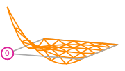
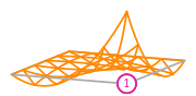
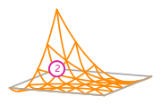
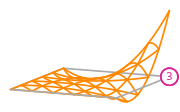
The basis functions of a second order Lagrange space on a quadrilateral (from DefElement, CC BY 4.0).

Uniqueness of basis functions

This means that we can use different basis functions to span the same polynomial spaces \(\mathcal{V}\) by choosing different dual basis functions \(l_i\).

An example of this is choosing different positioning of the dofs (non-equispaced) for Lagrange elements. See FEniCS: Variants of Lagrange Elements for more information.

An algorithmic approach for determining the basis functions based of the dual space is for instance given at Finite elements - analysis and implementation (Imperial College London).

Creating a finite element in FEniCSx

There is a large variety of finite elements: List of finite elements.

However, in today’s lecture, we will focus on the Lagrange elements.

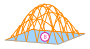
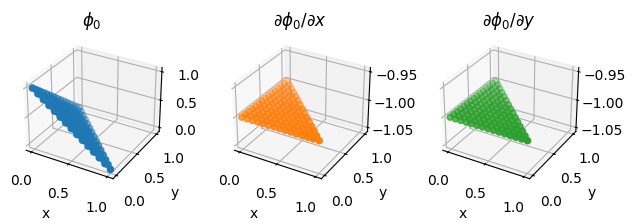
We start by considering the basis functions of a first order Lagrange element on a triangle:

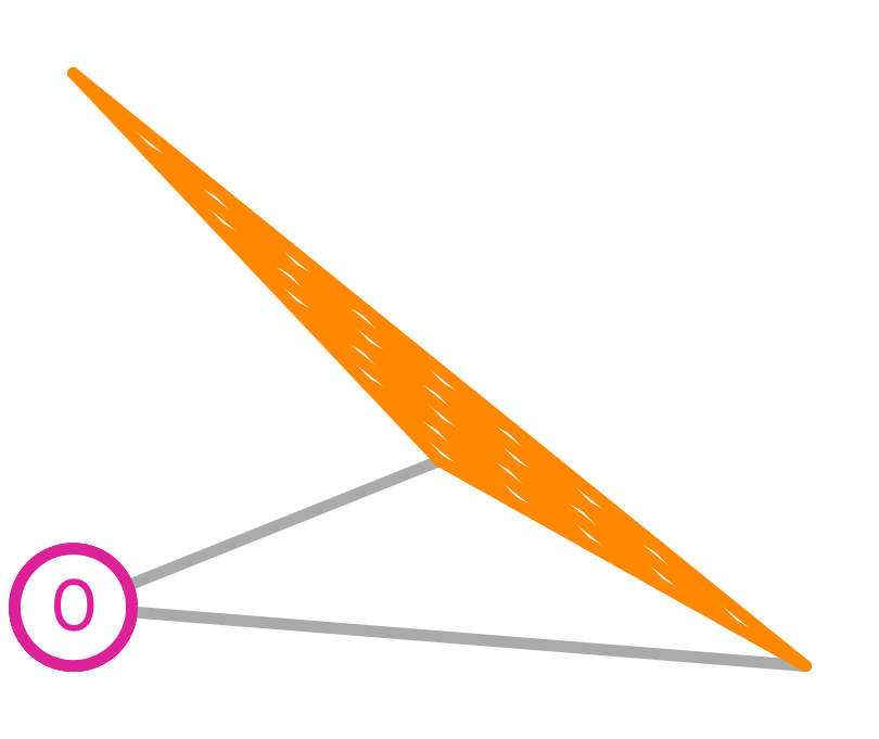
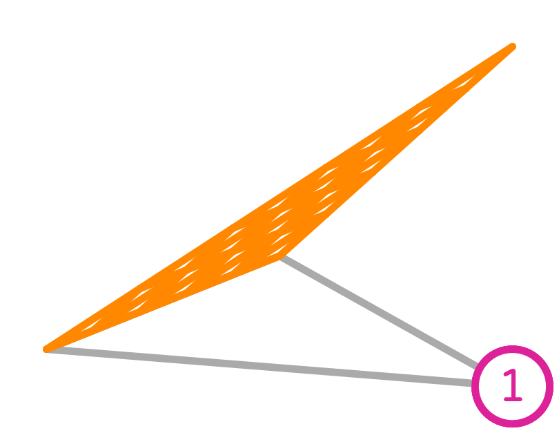
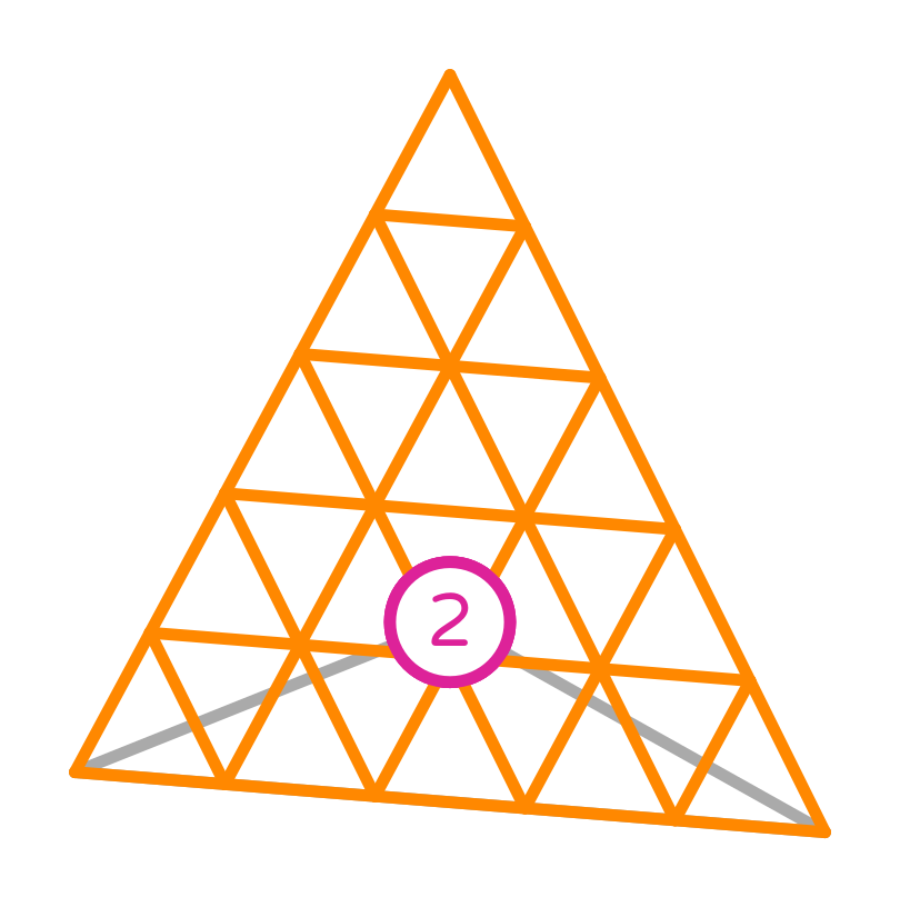
First order Lagrange basis functions

To symbolically represent this element, we use basix.ufl.element, that creates a representation of a finite element using Basix, which in turn can be used in the UFL.

import numpy as np

import basix.ufl

element = basix.ufl.element("Lagrange", "triangle", 1)

The three arguments we provide to Basix are the name of the element family, the reference cell we would like to use and the degree of the polynomial space.

Next, we will evaluate the basis functions at a certain set of points in the reference triangle. We call this tabulation and we use the tabulate method of the element object. The two input arguments are:

1. The number of spatial derivatives of the basis functions we want to compute.

2. A set of input points to evaluate the basis functions at as a numpy array of shape (num_points, reference_cell_dimension).

In this case, we want to compute the basis functions themselves, so we set the first argument to 0.

points = np.array([[0.,0.1], [0.3, 0.2]])
values = element.tabulate(0, points)

print(values)

[[[9.00000000e-01 5.55111512e-17 1.00000000e-01]
  [5.00000000e-01 3.00000000e-01 2.00000000e-01]]]

We can get the first order derivatives of the basis functions by setting the first argument to 1. Observe that the output we get from this command also includes the 0th order derivatives. Thus we note that the output has the shape (num_spatial_derivatives+1, num_points, num_basis_functions)

values = element.tabulate(1, points)

print(values)

[[[ 9.00000000e-01  5.55111512e-17  1.00000000e-01]
  [ 5.00000000e-01  3.00000000e-01  2.00000000e-01]]

 [[-1.00000000e+00  1.00000000e+00 -4.30845614e-17]
  [-1.00000000e+00  1.00000000e+00 -4.30845614e-17]]

 [[-1.00000000e+00  0.00000000e+00  1.00000000e+00]
  [-1.00000000e+00  0.00000000e+00  1.00000000e+00]]]

Visualizing the basis functions

Next, we create a short script for visualizing the basis functions on the reference element. We will for simplicity only consider first order derivatives and triangular or quadrilateral cells.

import matplotlib.pyplot as plt

def plot_basis_functions(element, M: int):
    """Plot the basis functions and the first order derivatives sampled at
    `M` points along each direction of an edge of the reference element.

    :param element: The basis element
    :param M: Number of points
    :return: The matplotlib instances for a plot of the basis functions
    """
    # We use basix to sample points (uniformly) in the reference cell
    points = basix.create_lattice(element.cell_type, M-1, basix.LatticeType.equispaced, exterior=True)

    # We evaluate the basis function and derivatives at the points
    values = element.tabulate(1, points)

    # Determine the layout of the plots
    num_basis_functions = values.shape[2]
    num_columns = values.shape[0]

    derivative_dir = ["x", "y"]
    figs = [plt.subplots(1, num_columns, layout='tight', subplot_kw={'projection': "3d"})
            for i in range(num_basis_functions)]
    colors = plt.rcParams["axes.prop_cycle"]()
    for i in range(num_basis_functions):
        _, axs = figs[i]
        [(ax.set_xlabel("x"),ax.set_ylabel("y")) for ax in axs.flat]
        for j in range(num_columns):
            ax = axs[j]
            ax.scatter(points[:, 0], points[:, 1], values[j, :, i], color=next(colors)["color"])
            if j > 0:
                ax.set_title(r"$\partial\phi_{i}/\partial {x_j}$".format(i="{"+f"{i}"+"}",
                                                                         x_j=derivative_dir[j-1]))
            else:
                ax.set_title(r"$\phi_{i}$".format(i="{"+f"{i}"+"}"))
    return figs

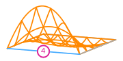
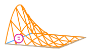
Basis functions sampled at random points

fig = plot_basis_functions(element, 15)

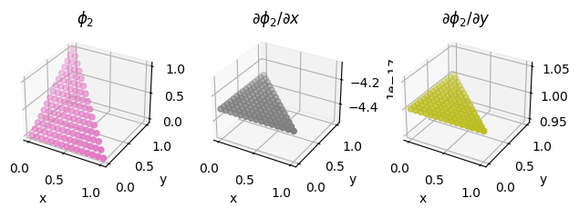
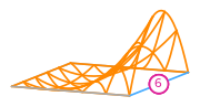
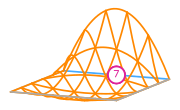
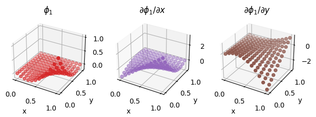
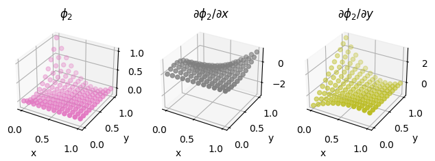
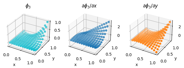
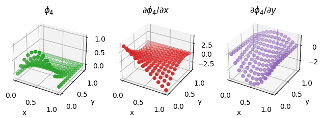
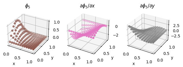
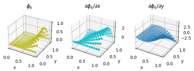
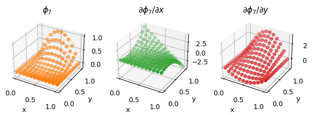
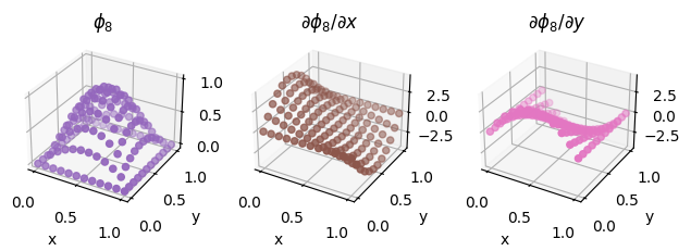
We also illustrate the procedure on a second order Lagrange element on a quadrilateral, as discussed above.

second_order_element = basix.ufl.element("Lagrange", "quadrilateral", 2, basix.LagrangeVariant.gll_warped)
fig = plot_basis_functions(second_order_element, 12)

Optional exercise

Using the plotting script above, try to plot basis functions of a high order quadrilateral element with different Lagrange variants. See: FEniCS: Variants of Lagrange Elements on how to add Lagrange variants to the element.

• Do you observe the same phenomenon on quadrilaterals as on intervals?

• What about triangles?

Hint: Try to increase the plotting resolution to 40.

Other finite elements

Not every function we want to represent is scalar valued. For instance, in fluid flow problems, the Taylor-Hood finite element pair is often used to represent the fluid velocity and pressure. For the velocity, each component (x, y, z) is represented with its own degrees of freedom in a Lagrange space.. We represent this by adding a shape argument to the basix.ufl.element constructor.

vector_element = basix.ufl.element("Lagrange", "triangle", 2, shape=(2,))

Basix allows for a large variety of extra options to tweak your finite elements, see for instance Variants of Lagrange elements for how to choose the node spacing in a Lagrange element.

To create the Taylor-Hood finite element pair, we use the basix.ufl.mixed_element

m_el = basix.ufl.mixed_element([vector_element, element])

There is a wide range of finite elements that are supported by ufl and basix. See for instance: Supported elements in basix/ufl.

Lower precision tabulation

In some cases, one might want to use a lower accuracy for tabulation of basis functions to speed up computations. This can be changed in basix by adding dtype=np.float32 to the element constructor.

low_precision_element = basix.ufl.element("Lagrange", "triangle", 1, dtype=np.float32)
points_low_precision = points.astype(np.float32)
basis_values = low_precision_element.tabulate(0, points_low_precision)
print(f"{basis_values=}\n   {basis_values.dtype=}")

basis_values=array([[[8.9999998e-01, 2.9802322e-08, 1.0000001e-01],
        [5.0000000e-01, 3.0000001e-01, 2.0000002e-01]]], dtype=float32)
   basis_values.dtype=dtype('float32')

We observe that elements that are close to zero is now an order of magnitude larger than its np.float64 counterpart.

[Cia02]

Philippe G. Ciarlet. The Finite Element Method for Elliptic Problems. Society for Industrial and Applied Mathematics, edition, 2002. doi:10.1137/1.9780898719208.