Diffusion of a Gaussian function#
Author: Jørgen S. Dokken
Let us now solve a more interesting problem, namely the diffusion of a Gaussian hill. We take the initial value to be
for \(a=5\) on the domain \([-2,2]\times[-2,2]\). For this problem we will use homogeneous Dirichlet boundary conditions (\(u_D=0\)).
The first difference from the previous problem is that we are not using a unit square.
We create the rectangular domain with dolfinx.mesh.create_rectangle().
import matplotlib as mpl
import pyvista
import ufl
import numpy as np

from petsc4py import PETSc
from mpi4py import MPI

from dolfinx import fem, mesh, io, plot
from dolfinx.fem.petsc import (
    assemble_vector,
    assemble_matrix,
    create_vector,
    apply_lifting,
    set_bc,
)
We define the time discretization parameters
t = 0.0  # Start time
T = 1.0  # Final time
num_steps = 50
dt = T / num_steps  # time step size
Next, we define the computational domain
nx, ny = 50, 50
domain = mesh.create_rectangle(
    MPI.COMM_WORLD,
    [np.array([-2, -2]), np.array([2, 2])],
    [nx, ny],
    mesh.CellType.triangle,
)
V = fem.functionspace(domain, ("Lagrange", 1))
Note that we have used a much higher resolution than before to better resolve features of the solution. We also easily update the intial and boundary conditions. Instead of using a class to define the initial condition, we simply use a function
def initial_condition(x, a=5):
    return np.exp(-a * (x[0] ** 2 + x[1] ** 2))


u_n = fem.Function(V)
u_n.name = "u_n"
u_n.interpolate(initial_condition)

# Create boundary condition
fdim = domain.topology.dim - 1
boundary_facets = mesh.locate_entities_boundary(
    domain, fdim, lambda x: np.full(x.shape[1], True, dtype=bool)
)
bc = fem.dirichletbc(
    PETSc.ScalarType(0), fem.locate_dofs_topological(V, fdim, boundary_facets), V
)
Time-dependent output#
To visualize the solution in an external program such as Paraview,
we create a an XDMFFile which we can store multiple solutions in.
The main advantage with an XDMFFile is that we only need to store the mesh once and that we can
append multiple solutions to the same grid, reducing the storage space.
The first argument to the XDMFFile is the communicator
which should be used to write data to file in parallel.
As we would like one output, independent of the number of processors,
we use the COMM_WORLD.
The second argument is the file name of the output file,
while the third argument is the state of the file,
this could be read ("r"), write ("w") or append ("a").
xdmf = io.XDMFFile(domain.comm, "diffusion.xdmf", "w")
xdmf.write_mesh(domain)
Define solution variable, and interpolate initial solution for visualization in Paraview
uh = fem.Function(V)
uh.name = "uh"
uh.interpolate(initial_condition)
xdmf.write_function(uh, t)
Variational problem and solver#
As in the previous example, we prepare objects for time dependent problems, such that we do not have to recreate data-structures.
u, v = ufl.TrialFunction(V), ufl.TestFunction(V)
f = fem.Constant(domain, PETSc.ScalarType(0))
a = u * v * ufl.dx + dt * ufl.dot(ufl.grad(u), ufl.grad(v)) * ufl.dx
L = (u_n + dt * f) * v * ufl.dx
Preparing linear algebra structures for time dependent problems#
We note that even if u_n is time dependent, we will reuse the same function for
f and u_n at every time step.
We therefore call dolfinx.fem.form() to generate assembly kernels for
the matrix and vector. This function creates a dolfinx.fem.Form.
We observe that the left hand side of the system, the matrix A
does not change from one time step to another, thus we only need to assemble it once.
We call A.assemble() to finalize the assembly process,
which means communicating local contributions from each process to other processes that shares the
same degrees of freedom.
However, the right hand side, which is dependent on the previous time step u_n,
we have to assemble it at every time step.
Therefore, we only create a vector b based on L,
which we will reuse at every time step.
A = assemble_matrix(bilinear_form, bcs=[bc])
A.assemble()
b = create_vector(fem.extract_function_spaces(linear_form))
Using petsc4py to create a linear solver#
As we have already assembled a into the matrix A, we can no longer
use the dolfinx.fem.petsc.LinearProblem class to solve the problem.
Therefore, we create a krylov subspace solver using PETSc,
assign the matrix A to the solver, and choose the solution strategy.
solver = PETSc.KSP().create(domain.comm)
solver.setOperators(A)
solver.setType(PETSc.KSP.Type.PREONLY)
solver.getPC().setType(PETSc.PC.Type.LU)
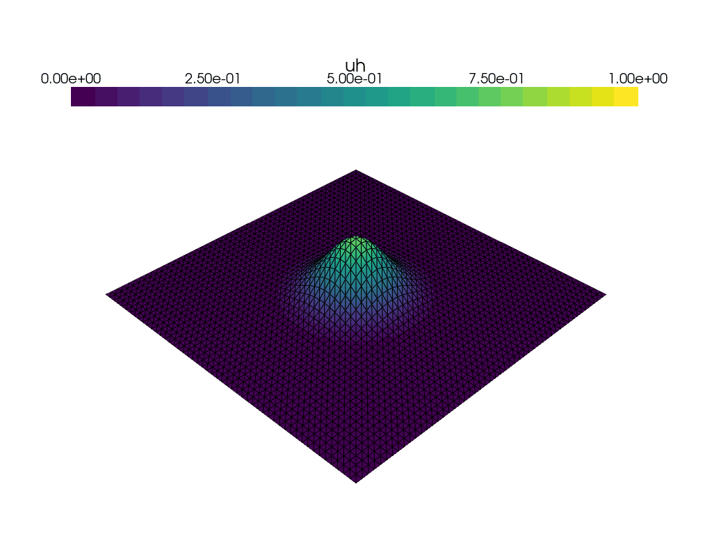
Visualization of time dependent problem using pyvista#
We use the DOLFINx plotting functionality, which is based on pyvista
to plot the solution at every \(15\)th time step.
We would also like to visualize a colorbar reflecting the minimal and maximum
value of \(u\) at each time step.
grid = pyvista.UnstructuredGrid(*plot.vtk_mesh(V))

plotter = pyvista.Plotter()
plotter.open_gif("u_time.gif", fps=10)

grid.point_data["uh"] = uh.x.array
warped = grid.warp_by_scalar("uh", factor=1)

viridis = mpl.colormaps.get_cmap("viridis").resampled(25)
sargs = dict(
    title_font_size=25,
    label_font_size=20,
    fmt="%.2e",
    color="black",
    position_x=0.1,
    position_y=0.8,
    width=0.8,
    height=0.1,
)

renderer = plotter.add_mesh(
    warped,
    show_edges=True,
    lighting=False,
    cmap=viridis,
    scalar_bar_args=sargs,
    clim=[0, max(uh.x.array)],
)
2026-07-07 12:19:04.049 ( 1.821s) [ 7FCF590F5140]vtkXOpenGLRenderWindow.:1460 WARN| bad X server connection. DISPLAY=
Updating the solution and right hand side per time step#
To be able to solve the variation problem at each time step,
we have to assemble the right hand side and apply the boundary condition before calling
solver.solve(b, uh.x.petsc_vec).
We start by resetting the values in b as we are reusing the vector at every time step.
The next step is to assemble the vector calling
dolfinx.fem.petsc.assemble_vector(b, L),
which means that we are assembling the linear form L(v) into the vector b.
Note that we do not supply the boundary conditions for assembly, as opposed to the left hand side.
This is because we want to use lifting to apply the boundary condition,
which preserves symmetry of the matrix \(A\) in the bilinear form \(a(u,v)=a(v,u)\) without Dirichlet boundary conditions.
Once we have performed the lifting, we accumulate values from degrees of freedom that are shared between processes
using b.ghostUpdate().
Finally, we apply the boundary condition to the fixed degrees of freedom with
dolfinx.fem.petsc.set_bc().
Next, we can solve the linear system and
update degrees of freedom shared between processors.
Finally, before moving to the next time step, we update the solution at the previous time step
to the solution at this time step.
for i in range(num_steps):
    t += dt

    # Update the right hand side reusing the initial vector
    with b.localForm() as loc_b:
        loc_b.set(0)
    assemble_vector(b, linear_form)

    # Apply Dirichlet boundary condition to the vector
    apply_lifting(b, [bilinear_form], [[bc]])
    b.ghostUpdate(addv=PETSc.InsertMode.ADD_VALUES, mode=PETSc.ScatterMode.REVERSE)
    set_bc(b, [bc])

    # Solve linear problem
    solver.solve(b, uh.x.petsc_vec)
    uh.x.scatter_forward()

    # Update solution at previous time step (u_n)
    u_n.x.array[:] = uh.x.array

    # Write solution to file
    xdmf.write_function(uh, t)
    # Update plot
    new_warped = grid.warp_by_scalar("uh", factor=1)
    warped.points[:, :] = new_warped.points
    warped.point_data["uh"][:] = uh.x.array
    plotter.write_frame()
plotter.close()
xdmf.close()
We destroy the PETSc objects to avoid memory leaks.
A.destroy()
b.destroy()
solver.destroy()
<petsc4py.PETSc.KSP at 0x7fcefd75a3e0>
Animation with Paraview#
We can also use Paraview to create an animation. We open the file in paraview with File->Open,
and then press Apply in the properties panel.
Then, we add a time-annotation to the figure, pressing: Sources->Alphabetical->Annotate Time
and Apply in the properties panel.
It Is also a good idea to select an output resolution, by pressing View->Preview->1280 x 720 (HD).
Then finally, click File->Save Animation, and save the animation to the desired format,
such as avi, ogv or a sequence of pngs. Make sure to set the frame rate to something sensible,
in the range of \(5-10\) frames per second.