Implementation#
Author: Antonio Baiano Svizzero and Jørgen S. Dokken
In this tutorial, you will learn how to:
Define acoustic velocity and impedance boundary conditions
Compute acoustic sound pressure for multiple frequencies
Compute the Sound Pressure Level (SPL) at a given microphone position
Test problem#
As an example, we will model a plane wave propagating in a tube. While it is a basic test case, the code can be adapted to way more complex problems where velocity and impedance boundary conditions are needed. We will apply a velocity boundary condition \(v_n = 0.001\) to one end of the tube (for the sake of simplicity, in this basic example, we are ignoring the point source, which can be applied with scifem) and an impedance \(Z\) computed with the Delaney-Bazley model, supposing that a layer of thickness \(d = 0.02\) and flow resistivity \(\sigma = 1e4\) is placed at the second end of the tube. The choice of such impedance (the one of a plane wave propagating in free field) will give, as a result, a solution with no reflections.
First, we create the mesh with gmsh, also setting the physical group for velocity and impedance boundary conditions and the respective tags.
import gmsh

gmsh.initialize()

# meshsize settings
meshsize = 0.02
gmsh.option.setNumber("Mesh.MeshSizeMax", meshsize)
gmsh.option.setNumber("Mesh.MeshSizeMax", meshsize)


# create geometry
L = 1
W = 0.1

gmsh.model.occ.addBox(0, 0, 0, L, W, W)
gmsh.model.occ.synchronize()

# setup physical groups
v_bc_tag = 2
Z_bc_tag = 3
gmsh.model.addPhysicalGroup(3, [1], 1, "air_volume")
gmsh.model.addPhysicalGroup(2, [1], v_bc_tag, "velocity_BC")
gmsh.model.addPhysicalGroup(2, [2], Z_bc_tag, "impedance")

# mesh generation
gmsh.model.mesh.generate(3)
Info    : Meshing 1D...
Info    : [  0%] Meshing curve 1 (Line)
Info    : [ 10%] Meshing curve 2 (Line)
Info    : [ 20%] Meshing curve 3 (Line)
Info    : [ 30%] Meshing curve 4 (Line)
Info    : [ 40%] Meshing curve 5 (Line)
Info    : [ 50%] Meshing curve 6 (Line)
Info    : [ 60%] Meshing curve 7 (Line)
Info    : [ 60%] Meshing curve 8 (Line)
Info    : [ 70%] Meshing curve 9 (Line)
Info    : [ 80%] Meshing curve 10 (Line)
Info    : [ 90%] Meshing curve 11 (Line)
Info    : [100%] Meshing curve 12 (Line)
Info    : Done meshing 1D (Wall 0.00110296s, CPU 0.000441s)
Info    : Meshing 2D...
Info    : [  0%] Meshing surface 1 (Plane, Frontal-Delaunay)
Info    : [ 20%] Meshing surface 2 (Plane, Frontal-Delaunay)
Info    : [ 40%] Meshing surface 3 (Plane, Frontal-Delaunay)
Info    : [ 60%] Meshing surface 4 (Plane, Frontal-Delaunay)
Info    : [ 70%] Meshing surface 5 (Plane, Frontal-Delaunay)
Info    : [ 90%] Meshing surface 6 (Plane, Frontal-Delaunay)
Info    : Done meshing 2D (Wall 0.0332048s, CPU 0.033432s)
Info    : Meshing 3D...
Info    : 3D Meshing 1 volume with 1 connected component
Info    : Tetrahedrizing 1285 nodes...
Info    : Done tetrahedrizing 1293 nodes (Wall 0.0156539s, CPU 0.013754s)
Info    : Reconstructing mesh...
Info    :  - Creating surface mesh
Info    :  - Identifying boundary edges
Info    :  - Recovering boundary
Info    : Done reconstructing mesh (Wall 0.0322988s, CPU 0.029814s)
Info    : Found volume 1
Info    : It. 0 - 0 nodes created - worst tet radius 2.85527 (nodes removed 0 0)
Info    : 3D refinement terminated (1746 nodes total):
Info    :  - 0 Delaunay cavities modified for star shapeness
Info    :  - 0 nodes could not be inserted
Info    :  - 6588 tetrahedra created in 0.0207364 sec. (317701 tets/s)
Info    : 0 node relocations
Info    : Done meshing 3D (Wall 0.0731105s, CPU 0.070776s)
Info    : Optimizing mesh...
Info    : Optimizing volume 1
Info    : Optimization starts (volume = 0.01) with worst = 0.0138257 / average = 0.769909:
Info    : 0.00 < quality < 0.10 :        18 elements
Info    : 0.10 < quality < 0.20 :        69 elements
Info    : 0.20 < quality < 0.30 :        66 elements
Info    : 0.30 < quality < 0.40 :        67 elements
Info    : 0.40 < quality < 0.50 :       150 elements
Info    : 0.50 < quality < 0.60 :       273 elements
Info    : 0.60 < quality < 0.70 :       913 elements
Info    : 0.70 < quality < 0.80 :      1842 elements
Info    : 0.80 < quality < 0.90 :      2090 elements
Info    : 0.90 < quality < 1.00 :      1095 elements
Info    : 152 edge swaps, 0 node relocations (volume = 0.01): worst = 0.300511 / average = 0.784453 (Wall 0.00255774s, CPU 0.002698s)
Info    : No ill-shaped tets in the mesh :-)
Info    : 0.00 < quality < 0.10 :         0 elements
Info    : 0.10 < quality < 0.20 :         0 elements
Info    : 0.20 < quality < 0.30 :         0 elements
Info    : 0.30 < quality < 0.40 :        67 elements
Info    : 0.40 < quality < 0.50 :       135 elements
Info    : 0.50 < quality < 0.60 :       271 elements
Info    : 0.60 < quality < 0.70 :       907 elements
Info    : 0.70 < quality < 0.80 :      1872 elements
Info    : 0.80 < quality < 0.90 :      2113 elements
Info    : 0.90 < quality < 1.00 :      1081 elements
Info    : Done optimizing mesh (Wall 0.00802258s, CPU 0.008174s)
Info    : 1746 nodes 9265 elements
Then we import the gmsh mesh with the dolfinx.io.gmsh module.
from mpi4py import MPI
from dolfinx import (
    fem,
    default_scalar_type,
    geometry,
    __version__ as dolfinx_version,
)
from dolfinx.io import gmsh as gmshio
from dolfinx.fem.petsc import LinearProblem
import ufl
import numpy as np
import numpy.typing as npt
from packaging.version import Version

mesh_data = gmshio.model_to_mesh(gmsh.model, MPI.COMM_WORLD, 0, gdim=3)
if Version(dolfinx_version) > Version("0.9.0"):
    domain = mesh_data.mesh
    assert mesh_data.facet_tags is not None
    facet_tags = mesh_data.facet_tags
else:
    domain, _, facet_tags = mesh_data
We define the function space for our unknown \(p\) and define the range of frequencies we want to solve the Helmholtz equation for.
V = fem.functionspace(domain, ("Lagrange", 1))

# Discrete frequency range
freq = np.arange(10, 1000, 5)  # Hz

# Air parameters
rho0 = 1.225  # kg/m^3
c = 340  # m/s
Boundary conditions#
The Delaney-Bazley model is used to compute the characteristic impedance and wavenumber of the porous layer, treated as an equivalent fluid with complex valued properties
where \(X = \frac{\rho_0 f}{\sigma}\).
With these, we can compute the surface impedance, that in the case of a rigid passive absorber placed on a rigid wall is given by the formula
Let’s create a function to compute it.
# Impedance calculation
def delany_bazley_layer(f, rho0, c, sigma):
    X = rho0 * f / sigma
    Zc = rho0 * c * (1 + 0.0571 * X**-0.754 - 1j * 0.087 * X**-0.732)
    kc = 2 * np.pi * f / c * (1 + 0.0978 * (X**-0.700) - 1j * 0.189 * (X**-0.595))
    Z_s = -1j * Zc * (1 / np.tan(kc * d))
    return Z_s


sigma = 1.5e4
d = 0.01
Z_s = delany_bazley_layer(freq, rho0, c, sigma)
Since we are going to compute a sound pressure spectrum, all the variables that depend on frequency (\(\omega\), \(k\) and \(Z\)) need to be updated in the frequency loop. To make this possible, we will initialize them as dolfinx constants. Then, we define the value for the normal velocity on the first end of the tube
omega = fem.Constant(domain, default_scalar_type(0))
k = fem.Constant(domain, default_scalar_type(0))
Z = fem.Constant(domain, default_scalar_type(0))
v_n = 1e-5
We also need to specify the integration measure \(ds\), by using ufl, and its built in integration measures
ds = ufl.Measure("ds", domain=domain, subdomain_data=facet_tags)
Variational Formulation#
We can now write the variational formulation.
The class LinearProblem is used to setup the PETSc backend and assemble the system vector and matrices.
The solution will be stored in a dolfinx.fem.Function, p_a.
p_a = fem.Function(V)
p_a.name = "pressure"

problem = LinearProblem(
    a,
    L,
    u=p_a,
    petsc_options={
        "ksp_type": "preonly",
        "pc_type": "lu",
        "pc_factor_mat_solver_type": "mumps",
    },
    petsc_options_prefix="helmholtz",
)
Computing the pressure at a given location#
Before starting our frequency loop, we can build a function that, given a microphone position, computes the sound pressure at its location. We will use the a similar method as in Deflection of a membrane. However, as the domain doesn’t deform in time, we cache the collision detection
class MicrophonePressure:
    def __init__(self, domain, microphone_position):
        """Initialize microphone(s).

        Args:
            domain: The domain to insert microphones on
            microphone_position: Position of the microphone(s).
                Assumed to be ordered as ``(mic0_x, mic1_x, ..., mic0_y, mic1_y, ..., mic0_z, mic1_z, ...)``

        """
        self._domain = domain
        self._position = np.asarray(
            microphone_position, dtype=domain.geometry.x.dtype
        ).reshape(3, -1)
        self._local_cells, self._local_position = self.compute_local_microphones()

    def compute_local_microphones(
        self,
    ) -> tuple[npt.NDArray[np.int32], npt.NDArray[np.floating]]:
        """
        Compute the local microphone positions for a distributed mesh

        Returns:
            Two lists (local_cells, local_points) containing the local cell indices and the local points
        """
        points = self._position.T
        bb_tree = geometry.bb_tree(self._domain, self._domain.topology.dim)

        cells = []
        points_on_proc = []

        cell_candidates = geometry.compute_collisions_points(bb_tree, points)
        colliding_cells = geometry.compute_colliding_cells(
            domain, cell_candidates, points
        )

        for i, point in enumerate(points):
            if len(colliding_cells.links(i)) > 0:
                points_on_proc.append(point)
                cells.append(colliding_cells.links(i)[0])

        return np.asarray(cells, dtype=np.int32), np.asarray(
            points_on_proc, dtype=domain.geometry.x.dtype
        )

    def listen(
        self, recompute_collisions: bool = False
    ) -> npt.NDArray[np.complexfloating]:
        if recompute_collisions:
            self._local_cells, self._local_position = self.compute_local_microphones()
        if len(self._local_cells) > 0:
            return p_a.eval(self._local_position, self._local_cells)
        else:
            return np.zeros(0, dtype=default_scalar_type)
The pressure spectrum is initialized as a numpy array and the microphone location is assigned
Frequency loop#
Finally, we can write the frequency loop, where we update the values of the frequency-dependent variables and solve the system for each frequency
for nf in range(0, len(freq)):
    k.value = 2 * np.pi * freq[nf] / c
    omega.value = 2 * np.pi * freq[nf]
    Z.value = Z_s[nf]

    problem.solve()
    p_a.x.scatter_forward()

    p_f = microphone.listen()
    p_f = domain.comm.gather(p_f, root=0)

    if domain.comm.rank == 0:
        assert p_f is not None
        p_mic[nf] = np.hstack(p_f)
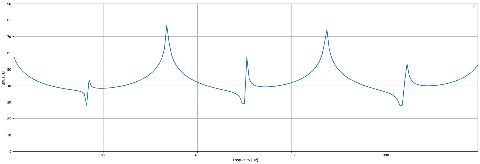
SPL spectrum#
After the computation, the pressure spectrum at the prescribed location is available. Such a spectrum is usually shown using the decibel (dB) scale to obtain the SPL, with the RMS pressure as input, defined as \(p_{rms} = \frac{p}{\sqrt{2}}\).
if domain.comm.rank == 0:
    import matplotlib.pyplot as plt

    fig = plt.figure(figsize=(25, 8))
    plt.plot(freq, 20 * np.log10(np.abs(p_mic) / np.sqrt(2) / 2e-5), linewidth=2)
    plt.grid(True)
    plt.xlabel("Frequency [Hz]")
    plt.ylabel("SPL [dB]")
    plt.xlim([freq[0], freq[-1]])
    plt.ylim([0, 90])
    plt.legend()
    plt.show()
/tmp/ipykernel_1267/2197754694.py:11: UserWarning: No artists with labels found to put in legend.  Note that artists whose label start with an underscore are ignored when legend() is called with no argument.
  plt.legend()