JIT options and visualization using Pandas

Author: Jørgen S. Dokken

In this chapter, we will explore how to optimize and inspect the integration kernels used in DOLFINx. As we have seen in the previous demos, DOLFINx uses the Unified form language to describe variational problems.

These descriptions have to be translated into code for assembling the right and left hand side of the discrete variational problem.

DOLFINx uses ffcx to generate efficient C code assembling the element matrices. This C code is in turn compiled using CFFI, and we can specify a variety of compile options.

We start by specifying the current directory as the location to place the generated C files, we obtain the current directory using pathlib

import pandas as pd
import seaborn
import time

from ufl import TestFunction, TrialFunction, dx, inner
from dolfinx.mesh import create_unit_cube
from dolfinx.fem.petsc import assemble_matrix
from dolfinx.fem import functionspace, form

from mpi4py import MPI
from pathlib import Path
from typing import Dict

cache_dir = f"{str(Path.cwd())}/.cache"
print(f"Directory to put C files in: {cache_dir}")

Directory to put C files in: /__w/dolfinx-tutorial/dolfinx-tutorial/chapter4/.cache

Next we generate a general function to assemble the mass matrix for a unit cube. Note that we use dolfinx.fem.form to compile the variational form. For codes using dolfinx.fem.petsc.LinearProblem, you can supply jit_options as a keyword argument.

def compile_form(space: str, degree: int, jit_options: Dict):
    N = 10
    mesh = create_unit_cube(MPI.COMM_WORLD, N, N, N)
    V = functionspace(mesh, (space, degree))
    u = TrialFunction(V)
    v = TestFunction(V)
    a = inner(u, v) * dx
    a_compiled = form(a, jit_options=jit_options)
    start = time.perf_counter()
    assemble_matrix(a_compiled)
    end = time.perf_counter()
    return end - start

We start by considering the different levels of optimization that the C compiler can use on the optimized code. A list of optimization options and explanations can be found here

optimization_options = ["-O1", "-O2", "-O3", "-Ofast"]

The next option we can choose is if we want to compile the code with -march=native or not. This option enables instructions for the local machine, and can give different results on different systems. More information can be found here

march_native = [True, False]

We choose a subset of finite element spaces, varying the order of the space to look at the effects it has on the assembly time with different compile options.

results = {"Space": [], "Degree": [], "Options": [], "Time": []}
for space in ["N1curl", "Lagrange", "RT"]:
    for degree in [1, 2, 3]:
        for native in march_native:
            for option in optimization_options:
                if native:
                    cffi_options = [option, "-march=native"]
                else:
                    cffi_options = [option]
                jit_options = {
                    "cffi_extra_compile_args": cffi_options,
                    "cache_dir": cache_dir,
                    "cffi_libraries": ["m"],
                }
                runtime = compile_form(space, degree, jit_options=jit_options)
                results["Space"].append(space)
                results["Degree"].append(str(degree))
                results["Options"].append("\n".join(cffi_options))
                results["Time"].append(runtime)

We have now stored all the results to a dictionary. To visualize it, we use pandas and its Dataframe class. To instpect the data in a Jupyter notebook, call the code below. If you are running this code in a script, you can use print(results_df) instead.

results_df = pd.DataFrame.from_dict(results)
results_df

	Space	Degree	Options	Time
0	N1curl	1	-O1\n-march=native	0.016477
1	N1curl	1	-O2\n-march=native	0.013306
2	N1curl	1	-O3\n-march=native	0.012766
3	N1curl	1	-Ofast\n-march=native	0.012694
4	N1curl	1	-O1	0.014798
...	...	...	...	...
67	RT	3	-Ofast\n-march=native	0.250178
68	RT	3	-O1	0.667445
69	RT	3	-O2	0.488837
70	RT	3	-O3	0.487357
71	RT	3	-Ofast	0.366428

72 rows × 4 columns

Next, we inspect the impact of the compiler option on each type of finite element family. To achieve this, we add an extra column to the dataframe, which combines the space and degree of the finite element.

seaborn.set(style="ticks")
seaborn.set(font_scale=1.2)
seaborn.set_style("darkgrid")
results_df["Element"] = results_df["Space"] + " " + results_df["Degree"]
elements = sorted(set(results_df["Element"]))
for element in elements:
    df_e = results_df[results_df["Element"] == element]
    g = seaborn.catplot(x="Options", y="Time", kind="bar", data=df_e, col="Element")
    g.fig.set_size_inches(16, 4)

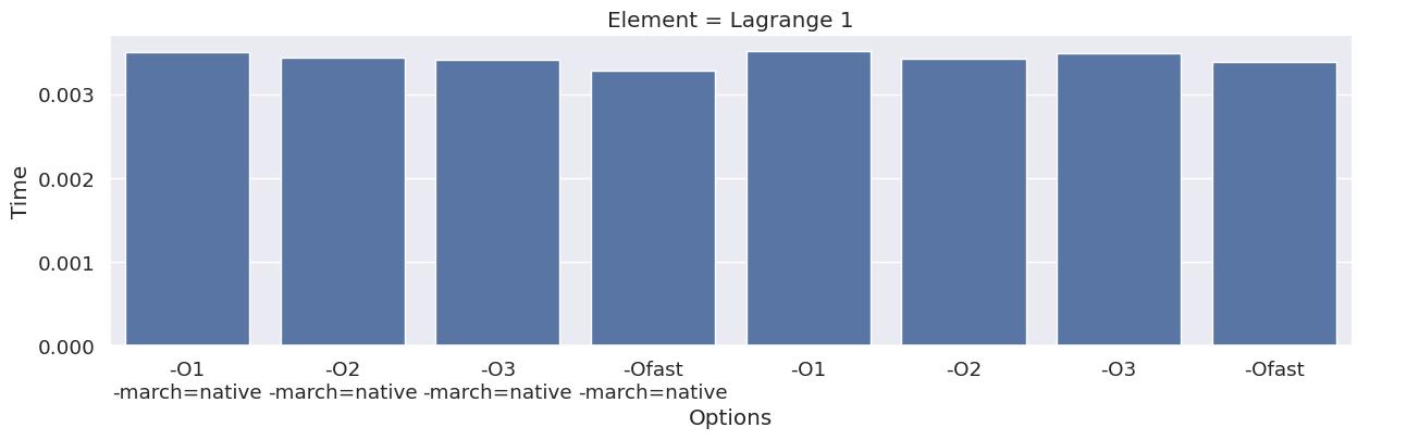
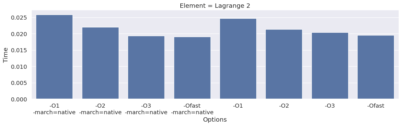
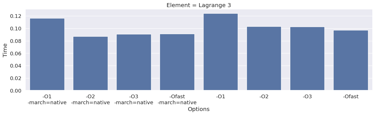
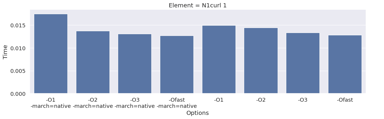
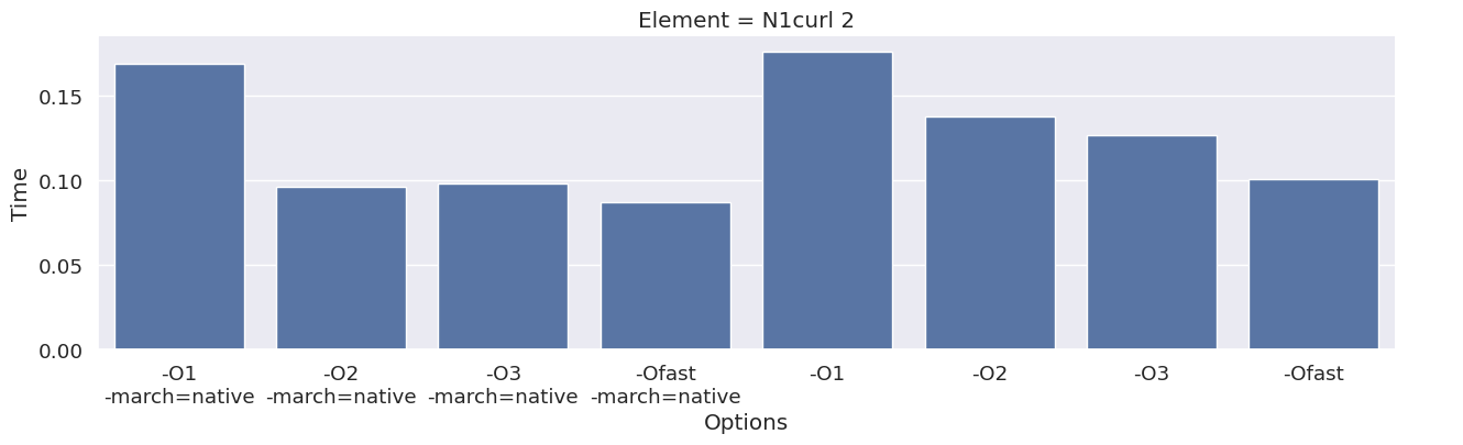
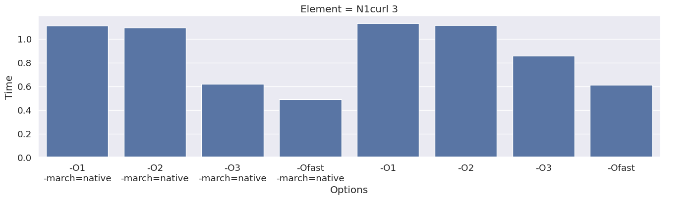
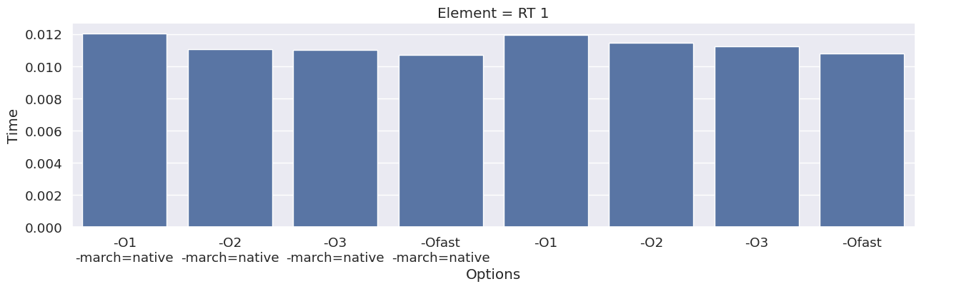
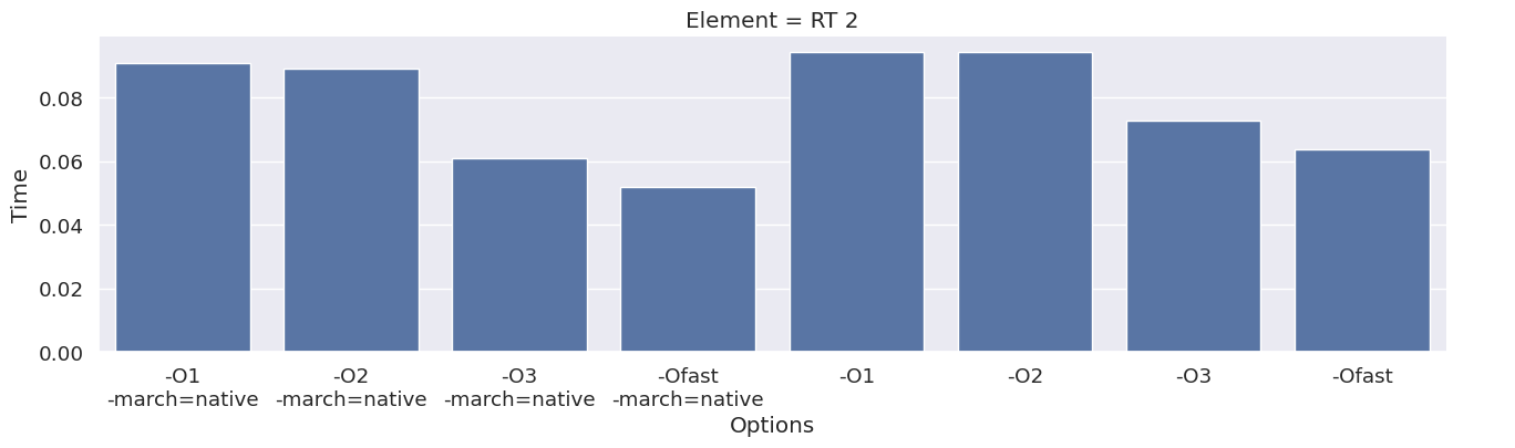
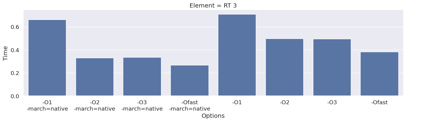
We observe that the compile time increases when increasing the degree of the function space, and that we get most speedup by using “-O3” or “-Ofast” combined with “-march=native”.