Custom Newton solvers#
Author: Jørgen S. Dokken
Newtons method, as used in the non-linear Poisson problem, is a way of solving a non-linear equation as a sequence of linear equations.
Given a function \(F:\mathbb{R}^M\mapsto \mathbb{R}^M\), we have that \(u_k, u_{k+1}\in \mathbb{R}^M\) is related as:
where \(J_F\) is the Jacobian matrix of \(F\).
We can rewrite this equation as \(\delta u_k = u_{k+1} - u_{k}\),
and
Problem specification#
We start by importing all packages needed to solve the problem.
import dolfinx
import dolfinx.fem.petsc
import matplotlib.pyplot as plt
import numpy as np
import pyvista
import ufl
from mpi4py import MPI
from petsc4py import PETSc
We will consider the following non-linear problem:
For this problem, we have two solutions, \(u=-x-1\), \(u=x+3\). We define these roots as python functions, and create an appropriate spacing for plotting these soultions.
def root_0(x):
    return 3 + x[0]


def root_1(x):
    return -1 - x[0]


N = 10
roots = [root_0, root_1]
x_spacing = np.linspace(0, 1, N)
We will start with an initial guess for this problem, \(u_0 = 0\).
Next, we define the mesh, and the appropriate function space and function uh to hold the approximate solution.
mesh = dolfinx.mesh.create_unit_interval(MPI.COMM_WORLD, N)
V = dolfinx.fem.functionspace(mesh, ("Lagrange", 1))
uh = dolfinx.fem.Function(V)
Definition of residual and Jacobian#
Next, we define the variational form, by multiplying by a test function and integrating over the domain \([0,1]\)
v = ufl.TestFunction(V)
x = ufl.SpatialCoordinate(mesh)
F = uh**2 * v * ufl.dx - 2 * uh * v * ufl.dx - (x[0] ** 2 + 4 * x[0] + 3) * v * ufl.dx
residual = dolfinx.fem.form(F)
Next, we can define the jacobian \(J_F\), by using ufl.derivative.
J = ufl.derivative(F, uh)
jacobian = dolfinx.fem.form(J)
As we will solve this problem in an iterative fashion, we would like to create the sparse matrix and vector containing the residual only once.
Setup of iteration-independent structures#
A = dolfinx.fem.petsc.create_matrix(jacobian)
L = dolfinx.fem.petsc.create_vector(dolfinx.fem.extract_function_spaces(residual))
Next, we create the linear solver and the vector to hold du.
solver.setOperators(A)
du = dolfinx.fem.Function(V)
We would like to monitor the evolution of uh for each iteration. Therefore, we get the dof coordinates, and sort them in increasing order.
i = 0
coords = V.tabulate_dof_coordinates()[:, 0]
sort_order = np.argsort(coords)
max_iterations = 25
solutions = np.zeros((max_iterations + 1, len(coords)))
solutions[0] = uh.x.array[sort_order]
We are now ready to solve the linear problem.
At each iteration, we reassemble the Jacobian and residual, and use the norm of the magnitude of the update (dx) as a termination criteria.
The Newton iterations#
i = 0
while i < max_iterations:
    # Assemble Jacobian and residual
    with L.localForm() as loc_L:
        loc_L.set(0)
    A.zeroEntries()
    dolfinx.fem.petsc.assemble_matrix(A, jacobian)
    A.assemble()
    dolfinx.fem.petsc.assemble_vector(L, residual)
    L.ghostUpdate(addv=PETSc.InsertMode.ADD_VALUES, mode=PETSc.ScatterMode.REVERSE)

    # Scale residual by -1
    L.scale(-1)
    L.ghostUpdate(addv=PETSc.InsertMode.INSERT_VALUES, mode=PETSc.ScatterMode.FORWARD)

    # Solve linear problem
    solver.solve(L, du.x.petsc_vec)
    du.x.scatter_forward()
    # Update u_{i+1} = u_i + delta u_i
    uh.x.array[:] += du.x.array
    i += 1

    # Compute norm of update
    correction_norm = du.x.petsc_vec.norm(0)
    PETSc.Sys.Print(f"Iteration {i}: Correction norm {correction_norm}")
    if correction_norm < 1e-10:
        break
    solutions[i, :] = uh.x.array[sort_order]
Iteration 1: Correction norm 29.41583333333333
Iteration 2: Correction norm 10.77679357571007
Iteration 3: Correction norm 2.0488925318207594
Iteration 4: Correction norm 0.08991946662079721
Iteration 5: Correction norm 0.0002277569702090273
Iteration 6: Correction norm 2.2114974378693033e-09
Iteration 7: Correction norm 1.2367958983836321e-15
We now compute the magnitude of the residual.
dolfinx.fem.petsc.assemble_vector(L, residual)
PETSc.Sys.Print(f"Final residual {L.norm(0)}")
A.destroy()
L.destroy()
solver.destroy()
Final residual 4.884981308350688e-16
<petsc4py.PETSc.KSP at 0x7f330edb2d40>
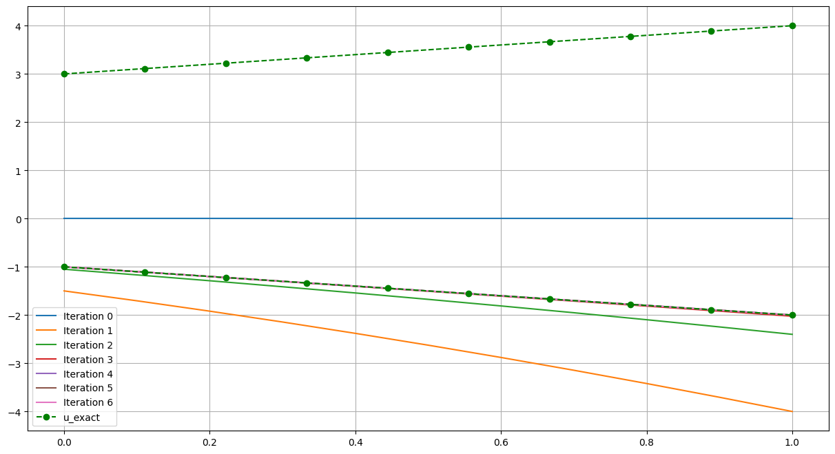
Visualization of Newton iterations#
We next look at the evolution of the solution and the error of the solution when compared to the two exact roots of the problem.
# Plot solution for each of the iterations
fig = plt.figure(figsize=(15, 8))
for j, solution in enumerate(solutions[:i]):
    plt.plot(coords[sort_order], solution, label=f"Iteration {j}")

# Plot each of the roots of the problem, and compare the approximate solution with each of them
args = ("--go",)
for j, root in enumerate(roots):
    u_ex = root(x)
    L2_error = dolfinx.fem.form(ufl.inner(uh - u_ex, uh - u_ex) * ufl.dx)
    global_L2 = mesh.comm.allreduce(dolfinx.fem.assemble_scalar(L2_error), op=MPI.SUM)
    PETSc.Sys.Print(f"L2-error (root {j}) {np.sqrt(global_L2)}")

    kwargs = {} if j == 0 else {"label": "u_exact"}
    plt.plot(x_spacing, root(x_spacing.reshape(1, -1)), *args, **kwargs)
plt.grid()
plt.legend()
L2-error (root 0) 5.033222956847167
L2-error (root 1) 1.4043333874306804e-16
<matplotlib.legend.Legend at 0x7f3305ffe4b0>
Newton’s method with DirichletBC#
In the previous example, we did not consider handling of Dirichlet boundary conditions. For this example, we will consider the non-linear Poisson-problem. We start by defining the mesh, the analytical solution and the forcing term \(f\).
def q(u):
    return 1 + u**2


domain = dolfinx.mesh.create_unit_square(MPI.COMM_WORLD, 10, 10)
x = ufl.SpatialCoordinate(domain)
u_ufl = 1 + x[0] + 2 * x[1]
f = -ufl.div(q(u_ufl) * ufl.grad(u_ufl))


def u_exact(x):
    return eval(str(u_ufl))
Next, we define the boundary condition bc, the residual F and the Jacobian J.
V = dolfinx.fem.functionspace(domain, ("Lagrange", 1))
u_D = dolfinx.fem.Function(V)
u_D.interpolate(u_exact)
fdim = domain.topology.dim - 1
domain.topology.create_connectivity(fdim, fdim + 1)
boundary_facets = dolfinx.mesh.exterior_facet_indices(domain.topology)
bc = dolfinx.fem.dirichletbc(
    u_D, dolfinx.fem.locate_dofs_topological(V, fdim, boundary_facets)
)

uh = dolfinx.fem.Function(V)
v = ufl.TestFunction(V)
F = q(uh) * ufl.dot(ufl.grad(uh), ufl.grad(v)) * ufl.dx - f * v * ufl.dx
J = ufl.derivative(F, uh)
residual = dolfinx.fem.form(F)
jacobian = dolfinx.fem.form(J)
Next, we define the matrix A, right hand side vector L and the correction function du
du = dolfinx.fem.Function(V)
A = dolfinx.fem.petsc.create_matrix(jacobian)
L = dolfinx.fem.petsc.create_vector(dolfinx.fem.extract_function_spaces(residual))
solver = PETSc.KSP().create(mesh.comm)
solver.setOperators(A)
solver.setType("preonly")
solver.getPC().setType("lu")
solver.getPC().setFactorSolverType("mumps")
solver.setErrorIfNotConverged(True)
Since this problem has strong Dirichlet conditions, we need to apply lifting to the right hand side of our Newton problem. We previously had that we wanted to solve the system:
we want \(u_{k+1}\vert_{bc}= u_D\). However, we do not know if \(u_k\vert_{bc}=u_D\). Therefore, we want to apply the following boundary condition for our correction \(\delta u_k\)
We therefore arrive at the following Newton scheme
i = 0
error = dolfinx.fem.form(
    ufl.inner(uh - u_ufl, uh - u_ufl) * ufl.dx(metadata={"quadrature_degree": 4})
)
L2_error = []
du_norm = []
while i < max_iterations:
    # Assemble Jacobian and residual
    with L.localForm() as loc_L:
        loc_L.set(0)
    A.zeroEntries()
    dolfinx.fem.petsc.assemble_matrix(A, jacobian, bcs=[bc])
    A.assemble()
    dolfinx.fem.petsc.assemble_vector(L, residual)

    # Compute b - alpha * J(u_D-u_(i-1))
    dolfinx.fem.petsc.apply_lifting(
        L, [jacobian], [[bc]], x0=[uh.x.petsc_vec], alpha=-1.0
    )
    L.ghostUpdate(addv=PETSc.InsertMode.ADD, mode=PETSc.ScatterMode.REVERSE)

    # Set du|_bc = - (u_{i-1}-u_D)
    dolfinx.fem.petsc.set_bc(L, [bc], uh.x.petsc_vec, -1.0)
    L.ghostUpdate(addv=PETSc.InsertMode.INSERT_VALUES, mode=PETSc.ScatterMode.FORWARD)

    # Compute negative residual
    L.scale(-1)

    # Solve linear problem
    solver.solve(L, du.x.petsc_vec)
    du.x.scatter_forward()

    # Update u_{i+1} = u_i + delta u_i
    uh.x.array[:] += du.x.array
    i += 1

    # Compute norm of update
    correction_norm = du.x.petsc_vec.norm(0)

    # Compute L2 error comparing to the analytical solution
    L2_error.append(
        np.sqrt(mesh.comm.allreduce(dolfinx.fem.assemble_scalar(error), op=MPI.SUM))
    )
    du_norm.append(correction_norm)
    PETSc.Sys.Print(
        f"Iteration {i}: Correction norm {correction_norm}, L2 error: {L2_error[-1]}",
        flush=True,
    )
    if correction_norm < 1e-10:
        break
Iteration 1: Correction norm 217.42583488321213, L2 error: 1.0094488413371545
Iteration 2: Correction norm 154.6085420034113, L2 error: 1.0258864066595137
Iteration 3: Correction norm 49.27248180384053, L2 error: 0.35418927062992456
Iteration 4: Correction norm 16.95612783044632, L2 error: 0.07129426316327732
Iteration 5: Correction norm 3.166818419654738, L2 error: 0.0045651615428112646
Iteration 6: Correction norm 0.17136876192941367, L2 error: 2.627050718275545e-05
Iteration 7: Correction norm 0.0008143256303865508, L2 error: 1.214917792790264e-09
Iteration 8: Correction norm 3.0496790845201666e-08, L2 error: 2.6816769692605512e-16
Iteration 9: Correction norm 8.750796124417366e-15, L2 error: 2.7214822409971685e-16
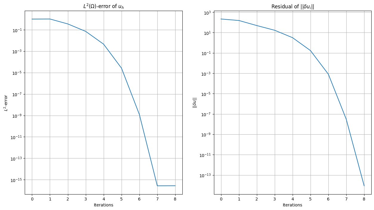
We plot the \(L^2\)-error and the residual norm (\(\delta u\)) per iteration
fig = plt.figure(figsize=(15, 8))
plt.subplot(121)
plt.plot(np.arange(i), L2_error)
plt.title(r"$L^2(\Omega)$-error of $u_h$")
ax = plt.gca()
ax.set_yscale("log")
plt.xlabel("Iterations")
plt.ylabel(r"$L^2$-error")
plt.grid()
plt.subplot(122)
plt.title(r"Residual of $\vert\vert\delta u_i\vert\vert$")
plt.plot(np.arange(i), du_norm)
ax = plt.gca()
ax.set_yscale("log")
plt.xlabel("Iterations")
plt.ylabel(r"$\vert\vert \delta u\vert\vert$")
plt.grid()
We compute the max error and plot the solution
error_max = domain.comm.allreduce(np.max(np.abs(uh.x.array - u_D.x.array)), op=MPI.MAX)
PETSc.Sys.Print(f"Error_max: {error_max:.2e}")
Error_max: 8.88e-16
u_topology, u_cell_types, u_geometry = dolfinx.plot.vtk_mesh(V)
u_grid = pyvista.UnstructuredGrid(u_topology, u_cell_types, u_geometry)
u_grid.point_data["u"] = uh.x.array.real
u_grid.set_active_scalars("u")
u_plotter = pyvista.Plotter()
u_plotter.add_mesh(u_grid, show_edges=True)
u_plotter.view_xy()
if not pyvista.OFF_SCREEN:
    u_plotter.show()
2026-07-07 12:35:38.119 ( 2.448s) [ 7F336AF48140]vtkXOpenGLRenderWindow.:1460 WARN| bad X server connection. DISPLAY=