Implementation#
Author: Jørgen S. Dokken
In this section, we will solve the deflection of the membrane problem. After finishing this section, you should be able to:
Create a simple mesh using the GMSH Python API and load it into DOLFINx
Create constant boundary conditions using a
geometrical identifierUse
ufl.SpatialCoordinateto create a spatially varying functionInterpolate a
ufl-Expressioninto an appropriate function spaceEvaluate a
dolfinx.fem.Functionat any point \(x\)Use Paraview to visualize the solution of a PDE
Creating the mesh#
To create the computational geometry, we use the Python-API of GMSH. We start by importing the gmsh-module and initializing it.
import gmsh

gmsh.initialize()
The next step is to create the membrane and start the computations by the GMSH CAD kernel,
to generate the relevant underlying data structures.
The first arguments of addDisk are the x, y and z coordinate of the center of the circle,
while the two last arguments are the x-radius and y-radius.
membrane = gmsh.model.occ.addDisk(0, 0, 0, 1, 1)
gmsh.model.occ.synchronize()
After that, we make the membrane a physical surface, such that it is recognized by gmsh when generating the mesh.
As a surface is a two-dimensional entity, we add 2 as the first argument,
the entity tag of the membrane as the second argument, and the physical tag as the last argument.
In a later demo, we will get into when this tag matters.
gdim = 2
gmsh.model.addPhysicalGroup(gdim, [membrane], 1)
1
Finally, we generate the two-dimensional mesh. We set a uniform mesh size by modifying the GMSH options.
gmsh.option.setNumber("Mesh.CharacteristicLengthMin", 0.05)
gmsh.option.setNumber("Mesh.CharacteristicLengthMax", 0.05)
gmsh.model.mesh.generate(gdim)
Info    : Meshing 1D...
Info    : Meshing curve 1 (Ellipse)
Info    : Done meshing 1D (Wall 0.000269227s, CPU 0.000479s)
Info    : Meshing 2D...
Info    : Meshing surface 1 (Plane, Frontal-Delaunay)
Info    : Done meshing 2D (Wall 0.0614466s, CPU 0.061687s)
Info    : 1550 nodes 3099 elements
Interfacing with GMSH in DOLFINx#
We will import the GMSH-mesh directly from GMSH into DOLFINx via the dolfinx.io.gmsh interface.
The dolfinx.io.gmsh module contains two functions
model_to_meshwhich takes in agmsh.modeland returns adolfinx.io.gmsh.MeshDataobject.read_from_mshwhich takes in a path to a.msh-file and returns adolfinx.io.gmsh.MeshDataobject.
The MeshData object will contain a dolfinx.mesh.Mesh,
under the attribute mesh.
This mesh will contain all GMSH Physical Groups of the highest topological dimension.
Note
If you do not use gmsh.model.addPhysicalGroup when creating the mesh with GMSH, it can not be read into DOLFINx.
The MeshData object can also contain tags for
all other PhysicalGroups that has been added to the mesh, that being
cell_tags, facet_tags,
ridge_tags and
peak_tags.
To read either gmsh.model or a .msh-file, one has to distribute the mesh to all processes used by DOLFINx.
As GMSH does not support mesh creation with MPI, we currently have a gmsh.model.mesh on each process.
To distribute the mesh, we have to specify which process the mesh was created on,
and which communicator rank should distribute the mesh.
The model_to_mesh will then load the mesh on the specified rank,
and distribute it to the communicator using a mesh partitioner.
from dolfinx.io import gmsh as gmshio
from dolfinx.fem.petsc import LinearProblem
from mpi4py import MPI

gmsh_model_rank = 0
mesh_comm = MPI.COMM_WORLD
mesh_data = gmshio.model_to_mesh(gmsh.model, mesh_comm, gmsh_model_rank, gdim=gdim)
assert mesh_data.cell_tags is not None
cell_markers = mesh_data.cell_tags
domain = mesh_data.mesh
We define the function space as in the previous tutorial
from dolfinx import fem

V = fem.functionspace(domain, ("Lagrange", 1))
Defining a spatially varying load#
The right hand side pressure function is represented using ufl.SpatialCoordinate and two constants,
one for \(\beta\) and one for \(R_0\).
import ufl
from dolfinx import default_scalar_type

x = ufl.SpatialCoordinate(domain)
beta = fem.Constant(domain, default_scalar_type(12))
R0 = fem.Constant(domain, default_scalar_type(0.3))
p = 4 * ufl.exp(-(beta**2) * (x[0] ** 2 + (x[1] - R0) ** 2))
Create a Dirichlet boundary condition using geometrical conditions#
The next step is to create the homogeneous boundary condition.
As opposed to the first tutorial we will use
locate_dofs_geometrical to locate the degrees of freedom on the boundary.
As we know that our domain is a circle with radius 1, we know that any degree of freedom should be
located at a coordinate \((x,y)\) such that \(\sqrt{x^2+y^2}=1\).
import numpy as np


def on_boundary(x):
    return np.isclose(np.sqrt(x[0] ** 2 + x[1] ** 2), 1)


boundary_dofs = fem.locate_dofs_geometrical(V, on_boundary)
As our Dirichlet condition is homogeneous (u=0 on the whole boundary), we can initialize the
dolfinx.fem.DirichletBC with a constant value, the degrees of freedom and the function
space to apply the boundary condition on. We use the constructor dolfinx.fem.dirichletbc().
bc = fem.dirichletbc(default_scalar_type(0), boundary_dofs, V)
Defining the variational problem#
The variational problem is the same as in our first Poisson problem, where f is replaced by p.
u = ufl.TrialFunction(V)
v = ufl.TestFunction(V)
a = ufl.dot(ufl.grad(u), ufl.grad(v)) * ufl.dx
L = p * v * ufl.dx
problem = LinearProblem(
    a,
    L,
    bcs=[bc],
    petsc_options={"ksp_type": "preonly", "pc_type": "lu"},
    petsc_options_prefix="membrane_",
)
uh = problem.solve()
Interpolation of a UFL-expression#
As we previously defined the load p as a spatially varying function,
we would like to interpolate this function into an appropriate function space for visualization.
To do this we use the class Expression.
The expression takes in any UFL-expression, and a set of points on the reference element.
We will use the interpolation points
of the space we want to interpolate in to.
We choose a high order function space to represent the function p, as it is rapidly varying in space.
Q = fem.functionspace(domain, ("Lagrange", 5))
expr = fem.Expression(p, Q.element.interpolation_points)
pressure = fem.Function(Q)
pressure.interpolate(expr)
Plotting the solution over a line#
We first plot the deflection \(u_h\) over the domain \(\Omega\).
from dolfinx.plot import vtk_mesh
import pyvista
Extract topology from mesh and create pyvista.UnstructuredGrid
topology, cell_types, x = vtk_mesh(V)
grid = pyvista.UnstructuredGrid(topology, cell_types, x)
Set deflection values and add it to plotter
grid.point_data["u"] = uh.x.array
warped = grid.warp_by_scalar("u", factor=25)

plotter = pyvista.Plotter()
plotter.add_mesh(warped, show_edges=True, show_scalar_bar=True, scalars="u")
if not pyvista.OFF_SCREEN:
    plotter.show()
else:
    plotter.screenshot("deflection.png")
2026-07-07 12:18:41.787 ( 0.810s) [ 7F4FDBF1F140]vtkXOpenGLRenderWindow.:1460 WARN| bad X server connection. DISPLAY=
We next plot the load on the domain
load_plotter = pyvista.Plotter()
p_grid = pyvista.UnstructuredGrid(*vtk_mesh(Q))
p_grid.point_data["p"] = pressure.x.array.real
warped_p = p_grid.warp_by_scalar("p", factor=0.5)
warped_p.set_active_scalars("p")
load_plotter.add_mesh(warped_p, show_scalar_bar=True)
load_plotter.view_xy()
if not pyvista.OFF_SCREEN:
    load_plotter.show()
else:
    load_plotter.screenshot("load.png")
Making curve plots throughout the domain#
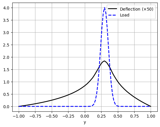
Another way to compare the deflection and the load is to make a plot along the line \(x=0\). This is just a matter of defining a set of points along the \(y\)-axis and evaluating the finite element functions \(u\) and \(p\) at these points.
tol = 0.001  # Avoid hitting the outside of the domain
y = np.linspace(-1 + tol, 1 - tol, 101)
points = np.zeros((3, 101))
points[1] = y
u_values = []
p_values = []
As a finite element function is the linear combination of all degrees of freedom,
\(u_h(x)=\sum_{i=1}^N c_i \phi_i(x)\) where \(c_i\) are the coefficients of \(u_h\) and \(\phi_i\)
is the \(i\)-th basis function, we can compute the exact solution at any point in \(\Omega\).
However, as a mesh consists of a large set of degrees of freedom (i.e. \(N\) is large),
we want to reduce the number of evaluations of the basis function \(\phi_i(x)\).
We do this by identifying which cell of the mesh \(x\) is in.
This is efficiently done by creating a bounding box tree<dolfinx.geometry.BoundingBoxTree
of the cells of the mesh,
allowing a quick recursive search through the mesh entities.
from dolfinx import geometry

bb_tree = geometry.bb_tree(domain, domain.topology.dim)
Now we can compute which cells the bounding box tree collides with using
dolfinx.geometry.compute_collisions_points().
This function returns a list of cells whose bounding box collide for each input point.
As different points might have different number of cells, the data is stored in
dolfinx.graph.AdjacencyList, where one can access the cells for the
ith point by calling links(i).
However, as the bounding box of a cell spans more of \(\mathbb{R}^n\) than the actual cell,
we check that the actual cell collides with the input point using
dolfinx.geometry.compute_colliding_cells(),
which measures the exact distance between the point and the cell
(approximated as a convex hull for higher order geometries).
This function also returns an adjacency-list, as the point might align with a facet,
edge or vertex that is shared between multiple cells in the mesh.
Finally, we would like the code below to run in parallel,
when the mesh is distributed over multiple processors.
In that case, it is not guaranteed that every point in points is on each processor.
Therefore we create a subset points_on_proc only containing the points found on the current processor.
cells = []
points_on_proc = []
# Find cells whose bounding-box collide with the the points
cell_candidates = geometry.compute_collisions_points(bb_tree, points.T)
# Choose one of the cells that contains the point
colliding_cells = geometry.compute_colliding_cells(domain, cell_candidates, points.T)
for i, point in enumerate(points.T):
    if len(colliding_cells.links(i)) > 0:
        points_on_proc.append(point)
        cells.append(colliding_cells.links(i)[0])
We now have a list of points on the processor, on in which cell each point belongs.
We can then call uh.eval and
pressure.eval to obtain the set of values for all the points.
points_on_proc = np.array(points_on_proc, dtype=np.float64)
u_values = uh.eval(points_on_proc, cells)
p_values = pressure.eval(points_on_proc, cells)
As we now have an array of coordinates and two arrays of function values,
we can use matplotlib to plot them
import matplotlib.pyplot as plt

fig = plt.figure()
plt.plot(
    points_on_proc[:, 1],
    50 * u_values,
    "k",
    linewidth=2,
    label="Deflection ($\\times 50$)",
)
plt.plot(points_on_proc[:, 1], p_values, "b--", linewidth=2, label="Load")
plt.grid(True)
plt.xlabel("y")
plt.legend()
<matplotlib.legend.Legend at 0x7f4f54f4f890>
If executed in parallel as a Python file, we save a plot per processor
plt.savefig(f"membrane_rank{MPI.COMM_WORLD.rank:d}.png")
<Figure size 640x480 with 0 Axes>
Saving functions to file#
As mentioned in the previous section, we can also use Paraview to visualize the solution.
import dolfinx.io
from pathlib import Path

pressure.name = "Load"
uh.name = "Deflection"
results_folder = Path("results")
results_folder.mkdir(exist_ok=True, parents=True)
with dolfinx.io.VTXWriter(
    MPI.COMM_WORLD, results_folder / "membrane_pressure.bp", [pressure], engine="BP4"
) as vtx:
    vtx.write(0.0)
with dolfinx.io.VTXWriter(
    MPI.COMM_WORLD, results_folder / "membrane_deflection.bp", [uh], engine="BP4"
) as vtx:
    vtx.write(0.0)