Smoothed TV image inpainting#
Authors: Jack Brockett and Jørgen S. Dokken
Download sources
This demo solves a variational image inpainting problem on the unit square. A synthetic image is masked on an irregular interior region, and the missing values are reconstructed using smoothed total variation (TV) regularization.
Problem Definition#
Let \(\Omega = [0,1]^2\) be the image domain. We define:
\(u_{\mathrm{true}}\): synthetic ground-truth image
\(m\): mask, equal to 1 on known data and 0 on the missing region
\(f = m u_{\mathrm{true}}\): observed incomplete image
\(u\): reconstructed image
We compute \(u\) by minimizing
The first term enforces agreement with the known image data, while the second term is a smoothed total variation regularization term. It promotes piecewise smooth solution and preserves edges \(\alpha\) and \(\beta\) control the balance between the data fidelity (fit to f) and smoothness. The parameter \(\varepsilon>0\) smooths the TV function so that it is differentiable and can be solved with Newton type methods
Discretization#
We discretize the problem using
a first order Lagrange finite element space
a triangular mesh of the unit square
Implementation#
We use a first-order Lagrange space on a triangular mesh
of the unit square.
The nonlinear problem is solved with
PETSc SNES through
NonlinearProblem.
from mpi4py import MPI

import matplotlib.pyplot as plt
import matplotlib.tri as mtri
import numpy as np

import ufl
from dolfinx import fem, mesh
from dolfinx.fem.petsc import NonlinearProblem
We discretize the domain \(\Omega =[0,1]^2\) using a triangular
mesh, where nx and ny control the resolution of the mesh.
nx = 128
ny = 128
msh = mesh.create_unit_square(MPI.COMM_WORLD, nx, ny)
We use first order Lagrange elements for discretizing the image. In this space, the DOFs are the values of u at mesh vertices the solution is continuous but has piecewise constant gradient
V = fem.functionspace(msh, ("Lagrange", 1))
Ground Truth image \(u_{true}\)#
We define a synthetic binary image
The square is defined as \(0.2<x<0.8, ~0.2<y<0.8\), which gives a piecewise-constant image with sharp edges
def true_image(x):
    """Define a binary image with a square in the center."""
    X = x[0]
    Y = x[1]

    # main square
    return ((X > 0.2) & (X < 0.8) & (Y > 0.2) & (Y < 0.8)).astype(np.float64)
Mask \(m(x,y)\)#
The mask defines which pixel are known and which are missing
We construct a mask with random “holes” inside the square
small circular regions are removed and set to 0
everywhere else remains known (1)
This creates a challenging inpainting problem as:
many small missing regions
irregular geometry
The solver must reconstruct these missing values using smoothness (TV regularization)
def mask_function(x):
    """Create a mask with random circular holes inside the square."""
    X = x[0]
    Y = x[1]
    # all pixels known
    mask = np.ones_like(X, dtype=np.float64)
    # number of speckles
    num_speckles = 25
    # random centers
    generator = np.random.Generator(
        np.random.MT19937(0)
    )  # random seed for reproducibility

    cx = generator.uniform(0.25, 0.75, num_speckles)
    cy = generator.uniform(0.25, 0.75, num_speckles)
    # random radii (small + varied)
    radii = generator.uniform(0.012, 0.035, num_speckles)
    # create holes. mask =0 inside circles
    for i in range(num_speckles):
        r2 = (X - cx[i]) ** 2 + (Y - cy[i]) ** 2
        mask[r2 < radii[i] ** 2] = 0.0
    return mask
We interpolate the exact image and the mask into the finite element space, and construct the observed damaged image, where \(u_{true}\) is our true image, \(m: \Omega \to \mathbb{R}\) is the mask, \(f: \Omega \to \mathbb{R}\) is the observed damaged image, and \(u:\Omega \to \mathbb{R}\) is the reconstructed image.
u_true = fem.Function(V, name="true_image")
u_true.interpolate(true_image)
m = fem.Function(V, name="mask")
m.interpolate(mask_function)
f = fem.Function(V, name="observed_image")
f.x.array[:] = m.x.array * u_true.x.array
u = fem.Function(V, name="reconstructed_image")
u.x.array[:] = f.x.array.copy()
We now define the nonlinear variational problem corresponding to the smoothed total variation regularised inpainting model.
The Euler-Lagrange equation for \(J(u)\) leads to the weak form Find \(u\in V\) such that
for all test functions \(v\). This is a nonlinear problem due to the TV term Total variation is usually defined as \(\vert\vert\nabla u\vert\vert\), but in practice one uses a smoothed version to allow for differentiation and Newton type solvers:
where # \(\varepsilon\) is the smoothing of the TV:
large \(\varepsilon\) smoother more like quadratic diffusion
small \(\varepsilon\) closer to true TV edge preserving
alpha = fem.Constant(msh, 0.003)
beta = fem.Constant(msh, 1.0)
eps = fem.Constant(msh, 1.0e-4)
Smoothed TV inpainting energy functional.
We define the energy J(u) and use ufl.derivative() to obtain
the residual form \(F(u; v)=0 \quad\forall v\in V\):
Taking the first variation gives the weak form F(u; v).
This formulation is based on total variation (TV) regularization for image denoising and inpainting Rudin et al. [ROF92], Shen and Chan [SC02].
A nonlinear PETSc problem is created and solved with a Newton line-search method, with an LU factorization for the linearized system \(F'(u_k) s= -F(u_k)\).
petsc_options = {
    "snes_type": "newtonls",
    "snes_linesearch_type": "bt",
    "snes_rtol": 1.0e-8,
    "snes_atol": 1.0e-8,
    "snes_max_it": 1000,
    "ksp_type": "preonly",
    "pc_type": "lu",
}

problem = NonlinearProblem(
    F,
    u,
    bcs=[],
    petsc_options_prefix="tv_inpainting_",
    petsc_options=petsc_options,
)

problem.solve()
Coefficient(FunctionSpace(Mesh(blocked element (Basix element (P, triangle, 1, gll_warped, unset, False, float64, []), (2,)), 0), Basix element (P, triangle, 1, gll_warped, unset, False, float64, [])), 3)
Model Validation and Results#
These diagnostics asses
whether the nonlinear Newton/SNES solve converged
whether the variational objective decreased
how accurate the reconstruction is globally and in the hole region
FEM Metrics Global number of degrees of freedom reports the size of the finite element discretization H1 seminorm error measures the gradient error
This is useful as TV regularization is gradient based. Smaller values mean the reconstruction recovers edge structure better
Reconstruction Errors Data fidelity (known region only):
measures the agreement with the known image data. Smaller values mean the reconstruction matches the observe pixels better.
TV seminorm
This is the regularization term in the objective Smaller values mean a smoother reconstruction
True error
Measures overall reconstruction accuracy
Hole error
Image quality metric PSNR (peak signal to noise ratio), standard imaging metric since the image range is [0,1], we use
Larger PSNR means better reconstruction quality
Newton Linesearch metrics Measure whether the nonlinear solve succeeded
we want a positive converged reason
a small final residual norm
a reasonable number of iterations
snes = problem.solver
reason = snes.getConvergedReason()
iters = snes.getIterationNumber()
final_residual = snes.getFunctionNorm()
Objective values Comparing the initial objective J(f) with the final objective J(u)
A decrease in the objective show that the nonlinear optimization improved the damaged image under the smoothed TV model
objective_value = 0.5 * float(beta) * data_error**2 + float(alpha) * tv_energy
if reason > 0:
    status = "converged"
else:
    status = "not converged"

u0 = fem.Function(V)
u0.x.array[:] = f.x.array.copy()

J0_data = fem.assemble_scalar(fem.form(m * (u0 - f) ** 2 * ufl.dx))
J0_data = msh.comm.allreduce(J0_data, op=MPI.SUM)

J0_tv = fem.assemble_scalar(
    fem.form(ufl.sqrt(ufl.inner(ufl.grad(u0), ufl.grad(u0)) + eps**2) * ufl.dx)
)
J0_tv = msh.comm.allreduce(J0_tv, op=MPI.SUM)

J0 = 0.5 * float(beta) * J0_data + float(alpha) * J0_tv
Printing statements for validation and metrics If on main process
if msh.comm.rank == 0:
    print("---Smoothed TV inpainting results---")

    print("--FEM Metrics--")
    print(f"Global DOFs: {num_dofs}")
    print(f"H1 seminorm error: {h1_semi_error}")

    print("--Newton Linesearch:--")
    print("-Optimization:-")
    print(f"Initial objective J(f): {J0:.4e}")
    print(f"Final objective J(u): {objective_value:.4e}")
    print(f"Relative decrease: {(J0 - objective_value) / J0:.2%}")

    print("-Solver convergence:-")
    print(f"SNES iteration: {iters}")
    print(f"SNES final residual norm: {final_residual:.4e}")
    print(f"SNES status: {status}")
    print(f"SNES converged reason: {reason}")

    print("---Reconstruction Quality:---")
    print(f"Data error (known region): {data_error:.4e}")
    print(f"TV seminorm: {tv_energy:.4e}")
    print(f"True L2 error: {true_error:.4e}")
    print(f"Hole error: {hole_error:.4e}")
    print(f"PSNR: {psnr:.2f} dB")
---Smoothed TV inpainting results---
--FEM Metrics--
Global DOFs: 16641
H1 seminorm error: 1.9251510135159864
--Newton Linesearch:--
-Optimization:-
Initial objective J(f): 1.7398e-02
Final objective J(u): 7.9366e-03
Relative decrease: 54.38%
-Solver convergence:-
SNES iteration: 430
SNES final residual norm: 2.6906e-09
SNES status: converged
SNES converged reason: 2
---Reconstruction Quality:---
Data error (known region): 4.7422e-02
TV seminorm: 2.2707e+00
True L2 error: 2.4220e-02
Hole error: 7.4629e-03
PSNR: 32.13 dB
Visualization#
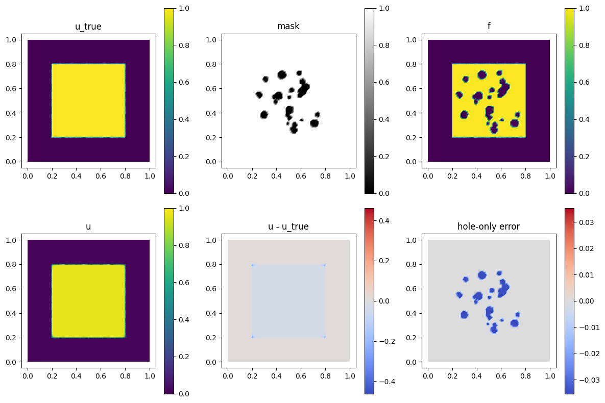
We construct fields that allow us to visually asses the quality of the reconstruction \(u-u_{true}\) is the global reconstruction error \((1-m)(u-u_{true})\) is the hole error, restricted to the missing regions
u_minus_u_true = fem.Function(V)
u_minus_u_true.x.array[:] = u.x.array - u_true.x.array

hole_error_field = fem.Function(V)
hole_error_field.x.array[:] = (1.0 - m.x.array) * (u.x.array - u_true.x.array)
FEM to matplotlib#
The solution u in FEM is represented by values at degrees of freedom (DOFs), not on a regular grid To plot in matplotlib
extract the coordinates of the DOFs
extract the function-space dofmap connectivity (triangles)
build a
Triangulationobject
This allows matplotlib to render the piecewise linear FEM solution
coords = V.tabulate_dof_coordinates()
x, y = coords[:, 0], coords[:, 1]

triangles = V.dofmap.list
triang = mtri.Triangulation(x, y, triangles)
Plotting
We use matplotlib.pyplot.tripcolor() to plot scalar fields defined on a
triangulated mesh shading= “flat” shows piecewise constant coloring per triangle
which better reflects the discrete FEM representations
def plot_field(ax, data, title, fig, cmap="viridis", vmin=0.0, vmax=1.0):
    """Plot a scalar field on a triangulated mesh."""
    im = ax.tripcolor(triang, data, shading="flat", cmap=cmap, vmin=vmin, vmax=vmax)
    ax.set_title(title)
    ax.set_aspect("equal")
    fig.colorbar(im, ax=ax)


fig, axes = plt.subplots(2, 3, figsize=(12, 8))
# $u_{true } $ground truth image
plot_field(axes[0, 0], u_true.x.array, "u_true", fig)
# m, mask with known (1) and missing (0) regions
plot_field(axes[0, 1], m.x.array, "mask", fig, cmap="gray")
# f is the damaged image
plot_field(axes[0, 2], f.x.array, "f", fig)
# u is the reconstructed image
plot_field(axes[1, 0], u.x.array, "u", fig)
# Global error
lim = np.max(np.abs(u_minus_u_true.x.array))
# $u-u_{true}$ is the global reconstruction error
plot_field(
    axes[1, 1],
    u_minus_u_true.x.array,
    "u - u_true",
    fig,
    cmap="coolwarm",
    vmin=-lim,
    vmax=lim,
)
# Hole only errors
lim = np.max(np.abs(hole_error_field.x.array))
# Hole only error restricted to the missing regions
plot_field(
    axes[1, 2],
    hole_error_field.x.array,
    "hole-only error",
    fig,
    cmap="coolwarm",
    vmin=-lim,
    vmax=lim,
)
plt.tight_layout()
plt.show()
References#
Leonid I. Rudin, Stanley Osher, and Emad Fatemi. Nonlinear total variation based noise removal algorithms. Physica D: Nonlinear Phenomena, 60(1):259–268, 1992. doi:10.1016/0167-2789(92)90242-F.
Jianhong Shen and Tony F. Chan. Mathematical Models for Local Nontexture Inpaintings. SIAM Journal on Applied Mathematics, 62(3):1019–1043, 2002. doi:10.1137/S0036139900368844.